EXERCISE 1: OBSIDIAN HYDRATION CHRONOLOGY

WORK IN GROUPS FEBRUARY 17; DISCUSSION: FEBRUARY 20;

The purpose of this exercise is to give you experience with creating an obsidian hydration chronology, and to use the resulting chronology to order a sequence of site use. Like seriation, obsidian hydration is a relative chronometer that works directly with artifacts. Some geologists and archaeologists have attempted to convert the hydration values (rind thickness values) into calendar years, but the conversions are not reliable. However, as a relative temporal tool, obsidian hydration works very well.

The principle behind obsidian hydration is simple. Obsidian cobbles absorb water at their surfaces so that over time a kind of rind forms on the surfaces. The longer obsidian has been absorbing water, the thicker the rind. Consequently, the thickness of the rind is an indicator of age: the thicker the rind, the older that piece is. On the other hand, the thinner the rind, the less time involved in water absorption. Now, here’s the really cool part: Flaking creates fresh surfaces which means that the hydration process begins again with the creation of a fresh surface. The implication here is that we can determine (on a relative scale) when an obsidian flake was removed or when a cobble was worked. Thus, we can create a relative order of obsidian use. So for instance, pieces of obsidian that were flaked by Paleo-indians will have much thicker rinds than pieces that flaked by Puebloans 400 years ago.

Rind thickness values are measured in microns (μ). A micron is .001 of a millimeter (tiny measurements!). A micron value of 1.0 is thinner than micron value of 10.0 In other words, as the value becomes larger, the thickness of the rind is greater.

Several factors affect the rind thickness or our ability to construct a chronology. First not all types of obsidian absorb water at the same rate. Before we can measure hydration rinds, we must determine the source of the obsidian. Because the rate of absorption varies by source, obsidian from two sources that have the same value are not the same age. The upside of this problem is that if you control for source, the same hydration value from two pieces of obsidian from different sites is approximately the same age. Thus, two pieces with a micron value of 4.1 from a single source is the same age. The second problem is a consequence of obsidian itself. Because obsidian is such an excellent tool stone, it can be reused. In other words, a spear point that was made 10,000 years ago may have been dropped and later picked up and reshaped. The reshaping resets the hydration clock to zero. Alternatively, the spear point may not have been reshaped. It may simply have been used. The use of the spear point will not change the hydration value, but the hydration value of this object may be very different than the other hydration values from the site. Because obsidian can be reused, to create a chronology, you need large samples of obsidian flakes or tools where source and rind thickness have been calculated.

In this exercise, there are three sites located in the Jemez Mountains of New Mexico (where there are rich obsidian deposits). We have made surface collections from these sites. Each site has about 500 flaked artifacts. Obsidian artifacts constitute about 25% of each assemblage. The sites do not appear to have been villages. Instead, the nature and type of artifacts suggests that these sites were visited periodically by mobile hunter-gatherers. We have separated the obsidian artifacts, and have selected between 100 and 160 obsidian flakes from each site to source and to calculate the rind values. We have learned that all the obsidian flakes derive from a single source (Cerro del Medio, one of the sources in the Jemez Mountains), and we have just received the information on rind thickness for all the flakes from each of three sites.

TASKS

1. Create counts of hydration bands by lumping smaller values into larger ones. Appended to this document (at the end of this handout) are the hydration values of the obsidian flakes from three sites. The column named count identifies the number of flakes that measured to that hydration value. The values are arranged in descending order. The smallest hydration values are on top of the spreadsheet. The largest are at the bottom. The values are in tenths of microns, e.g., 1.2, or 4.3.

To complete the first part of this exercise, you will have to use a spread sheet program like Excel which has both a spread sheet function and a chart function. Before you can temporally order the sites by the obsidian values, you must create larger micron units based on rind values. These larger micro value units are temporal units.

For each site, you are to sum all the counts of obsidian flakes between whole numbers, 1.0-1.9, 2.0-2.9, 3.0-3.9 etc. (See example) You repeat this process for all counts from each site. Essentially, what you are doing here is lumping smaller values into larger rind thickness categories. Record your new data in rows and column on a new spread sheet.

Example:

OBSERVED HYDRATION VALUES
micron	counts
1	5
1.4	8
1.5	5
1.7	4
1.8	4

2.1	6
2.4	3
2.5	3
2.8	2

5	1
GROUPED VALUES
grouped	counts
5.0-5.9	1
4.0-4.9	0
3.0-3.9	0
2.0-2.9	14
1.0-1.9	26

2) Once you have created larger temporal units by site, you are ready to graph the distribution of hydration values by site. To do this, you need to create a new work sheet. The first column should be a master list of obsidian microns by whole numbers, 1-1.9, 2-2.9, 3-3.9, etc. The next 3 columns should be the sum by site of obsidian flakes in each temporal interval. For instance,

the Hughes site has 39 flakes with measurements between 1.0 and 1.9 microns. You are then ready to create your graphs.

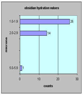
The purpose of the graphs are to show you the chronology of obsidian use through time. In the example below, I selected the grouped values, and then went to the Insert menu, and selected Charts bar. Simply follow the menu. The resulting graph displays the counts of hydration values. As you can see in the example, there are lots of values between 1.0 and 1.9. There are also values between 2.0 and 2.9. There is one outlier value between 5.0 and 5.9 microns. This outlier may be the result of picking up an old obsidian flake or perhaps, some forager visited this place in the distance past. In other words, there is one strong period of use that is quite recent, and one outlier.

3. Create graphs of obsidian use for each of the three sites. You can then compare the values of obsidian hydration rinds across sites to determine the chronology of visitation. After you have examined the three graphs, please answer the following questions

Questions

You must write out your answers to the question. We want you to turn in both the work sheets with the final write up and graphs.

For the purpose of this exercise, we will consider each micron width (1-1.9; 2.0-2.9, etc.) to be a separate episode of use. If thickness values are continuous between whole numbers (as in the example above [ 2.9- 1.0]), you can assume that the site was reused continuously across the temporal interval 1-2.9. In essence, you are going to use the micron widths as intervals of time. What you are trying to do here is to develop peaks of use at each site.

1. For each site, collapse the smaller micron values into whole numbers, and create a bar graph of each site. Then, decide and describe how many episodes of use are present at each site. (You can assume that breaks in the distribution of whole micron values indicate no visitation to the site.) In other words, how many episodes of use are represented at each site? Does the Hughes site have one or more than one episode of use. What are the micron values that relate to these use periods. What about the Steffen site and the Plet site?

2. . Examine the episodes of site use across the three sites. Which site has the most recent use, and which site has the longest episodes of use? How did you arrive at these conclusions?

3. Describe the chronology of site use based on the micron values from the 3 sites. Do these three sites have the same periods of use, or are there some temporal overlaps, but each site has distinctly different temporal peaks?

4. Are there some odd or unexpected micron values (called outliers) at any of these sites? How might you account for these outliers?

THE FOLLOWING IS THE DATA SET TO USE FOR THIS EXERCISE:

SITE 1:	HUGHES SITE	SITE 2	SMITH SITE	SITE 3	PLET
Micron Meas.	Value	Micron Meas	Value	Micron Meas	Value

1	9	1.7	1	1	2
1.4	7	2	4	2.4	4
1.5	5	2.3	1	2.5	5
1.6	8	2.4	4	2.7	3
1.8	9	2.5	4	2.9	5
1.9	1	2.9	16	3.1	13
2	13	3.1	11	3.4	11
2.1	3	3.2	1	5.1	5
2.3	12	3.3	8	5.2	3
6.3	5	3.4	7	5.3	2
6.4	2	3.8	15	5.4	3
6.5	5	3.9	14	5.8	8
6.7	4	4.1	17	5.9	12
6.9	6	4.3	12	6.1	6
7	3	4.6	16	6.3	7
7.1	3	4.7	13	9.1	1
7.4	7	5	7	9.4	3
7.5	4	5.4	3	9.5	1
7.7	3	5.7	3	9.8	8
7.8	2	6.2	2	9.9	7
7.9	6	6.3	2	10.1	14
8	1	6.6	1	10.2	13
9.1	2	13	2	10.4	7
				10.8	5
				11	8
Total	120		164		156