Code-along format:

In parallel with the main sessions of the course, the optional “code-along” track will see the participants build their own numerical matrix product states library based on the literature presented during the course sessions. The code-along track is intended to provide the participants with intuition and hands-on experience on the numerical implementation of the matrix product states formalism. Following the completion of the course, the participants can then use their own MPS library or one of the freely available tensor networks libraries (e.g., iTensor) for numerical simulations.

Code-along track office hours with Philip Blocher will be held in person on Wednesdays 10am-12pm MDT at PAIS room 2210 and virtually on Wednesdays 1pm-2.30pm MDT using Zoom (ID: 976 1820 8213, PW: Tensor@UNM). For those participating in the code-along track, Philip will be available for help/discussions upon arrangement via email (blocher@unm.edu), via the CQuIC Slack, or in person at PAIS 2526.

Participants of the code-along track are free to use any programming language, bearing in mind that the matrix product states formalism will include heavy use of linear algebra functions such as matrix addition, matrix multiplication, Kronecker tensor products of matrices, and singular value decompositions. Philip has written his own library in MATLAB and has experience using C++ and python.

Code-along goals:

The following is a list of the functions that we need to implement in order to create our own numerical matrix product states (MPS) library. The functions are listed in order of increasing complexity / dependence on previous functions, and it is recommended to implement the functions in the order presented here. For each function one or several suggested exercises are given to verify that the function is working as intended.

We suggest using the transverse field Ising model as our physical model. The aim of this code-along track will then be to have a numerical MPS library which can implement the time evolution of a 1D model, in our case the transverse field Ising model, with everything that this entails. Participants are – of course – welcome to choose any other physical model for their code, though a model consisting of a 1D chain of qubits (or qudits) is preferable. An example could be the Bose-Hubbard model in 1D.

Finally, Philip’s personal MPS library written for MATLAB is available on Github for reference/inspiration. Note that Philip’s MPS library is a heavily modified version of the library that we will implement here, and that functions in Philip’s MPS library may therefore include features that are beyond the scope of this code-along track – ignore these.

The transverse field Ising model Hamiltonian reads

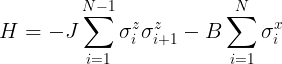
where J is the strength of the nearest-neighbor spin-spin interaction, and B is the strength of the transverse magnetic field.

Function 1: generate a random MPS

§ Intent: This function should generate an MPS object whose constituent matrices are random matrices. The constituent matrices should have the correct dimensions according to the text below Eq. (37) in [Schollwöck2011]: (1 x d), (d x d²), … , (d x 1), where d is the number of physical degrees of freedom per site (d = 2 for qubits).

§ The implementation of this function is intended to help us figure out how to create the MPS object numerically. For each site in our 1D lattice we need to store a number of matrices equal to the physical degrees of freedom for that site. One idea for an MPS object would be to create a 2D array of size (d x L), where the row index corresponds to the physical index of each MPS tensor, and where the column index corresponds to the MPS sites / tensors.

Function 2: return the state vector for any given MPS

§ Intent: This function should calculate each state vector entry by multiplying together (contracting) the appropriate constituent matrices of the MPS. We will need to create an indexing system that reads off all permutations of matrix multiplications without being hardcoded for a particular number of sites N.

§ Note that for a given choice of physical indices sigma1, sigma2, etc., this function contracts the MPS tensor network to obtain the tensor network value, which corresponds to the state vector entry.

§ Exercise: Test that the method works (up to not being able to verify the state vector entries) by applying Function 2 to a random MPS generated by Function 1. Once Function 3 is implemented, test that Function 2 applied to the output MPS of Function 3 returns the correct state vector.

Function 3: decomposition algorithm that creates a ‘left-canonical’ MPS from any input state vector

§ Intent: This function should take as input a state written as a state vector and output the corresponding ‘left-canonical’ MPS.

§ A good place to start would be to consider the algorithm presented in Eqs. (18-23) of [Schollwöck2013].

§ Exercise: Create a random state vector and run the MPS decomposition algorithm on it. Use Function 2 to check that you recover the original state vector from the MPS. Is the MPS that you have created normalized? At which point during the algorithm do we find the state norm of the input state?

§ Exercise: The algorithm presented in Eqs. (18-23) of [Schollwöck2013] should yield a left-canonical MPS. Check that this is the case for the MPS created through the decomposition algorithm.

§ Exercise: Create the MPS representation of both the “all spin-up along z” state |+z> = (tensor product of individual spins pointing along +z), and the “all spin-up along x” state |+x> = (tensor product of individual spins pointing along +x).

Function 4: bring an arbitrary MPS onto either ‘left-canonical’ or ‘right-canonical’ form (also doubles as a renormalization algorithm)

§ Intent: When manipulating MPS (say, during time evolution), it becomes necessary to be able to bring the MPS back onto so-called canonical forms. This function will take any MPS and bring it onto a left- or right-canonical form. The function will also serve as a renormalization algorithm, allowing us to renormalize our MPS if needed.

§ The (re)normalization of MPS is described in chapter 4 of [Schollwöck2013]. Implement a function that can bring an arbitrary MPS onto ‘left-canonical’ form using, e.g., the procedure described in Eqs. (35-41) of [Schollwöck2013]. Extend the function so that it can also bring an arbitrary MPS onto ‘right-canonical’ form, and use an input variable to choose whether we bring the MPS onto left- or right-canonical form (we will use both forms later!)

§ Exercise: Check that the constituent matrices satisfy the requirements for being left(right)-normalized after the MPS has been brought onto left(right)-canonical form, and that the MPS is normalized using Function 2 (or Function 5 once it is implemented).

§ Exercise: We can change the norm of an MPS by multiplying all matrices on one site by a scalar. Create an MPS using Function 3, then multiply all matrices on the first site by a scalar. Apply our renormalization algorithm to this ‘unnormalized’ MPS and check that the resulting MPS is renormalized using Function 2 (or Function 5 once it is implemented).

Function 5: calculate the overlap between two MPS

§ Intent: This function calculates the overlap <Φ|Ψ> between two MPS |Ψ>, |Φ >. One place to find the discussion of overlaps is in chapter 6 of [Schollwöck2013].

§ Note: There is a numerically optimal way of contracting the tensor network <Φ|Ψ>, which is described in the unnumbered equation between Eq. (48) and Eq. (49) in [Schollwöck2013].

§ Exercise: Check that the overlap between the (normalized) MPS |Ψ> and itself yields 1. What is the overlap between |+z> and |+x> defined above?

Function 6: generate a random MPO

§ Intent: Just as we did with the MPS in Function 1, we start our implementation of matrix product operators (MPOs) by first implementing a function that returns an MPO whose constituent matrices are random matrices of appropriate sizes.

§ What is the structure of the MPO? Remember that we need two physical indices for each site, in contrast to one index per site for the MPS.

§ What are the maximum matrix sizes (MPO bond dimensions) allowed for each lattice site? The MPO bond dimensions scale differently from MPS bond dimensions, but how?

Function 7: apply an MPO to an MPS

§ Intent: This function should apply an MPO Q to an MPS |Ψ>. The resulting object |QΨ> is itself an MPS whose matrices are combinations of the original MPO and MPS matrices.

§ One place to find the description of this algorithm is in chapter 5 of [Schollwöck2011]. Schollwöck does not state so in [Schollwöck2011], but the single-site matrix products are in fact Kronecker tensor product. This realization should make the code implementation easier and avoid having to implement several for-loops!

§ Exercise: Check that this function works by creating a random MPO using Function 6 and applying it to an MPS of your choice. Verify that the resulting matrices have the correct dimensions.

§ Exercise: Once Function 9 is online, we can check that Function 7 works as intended by creating the MPO for a known operator and calculate its expectation value in a known MPS using Function 5.

§ Exercise: It is also quite easy to manually create MPO-representations of single-site operators by first creating an MPO that has identities (δ_{σ σ’}) on all sites, and then replacing this identity with the desired operator on a single site. Try doing so with, e.g., S_x and S_y on one site, and check that Function 7 works as intended for these operators. Inspiration can be found in Philip’s personal MPS library on Github if you get stuck.

§ Note that applying an MPO to an MPS causes the MPS bond dimensions to grow!

Function 8: compress the bond dimensions of an MPS according to a specified maximum bond dimension χ and a single-site compression error ε.

§ Intent: Applying an MPO to an MPS will increase the bond dimension of the MPS, as we saw in our implementation of Function 7. Thus, we need a method of compressing the MPS bond dimensions (also known as “truncating the MPS bond dimensions”). Implementing this function will give us one particular way of doing so using singular value decompositions, the other way being “variational (iterative) bond dimension compression”. The function should take as input a specified maximum bond dimension χ and a tolerable single-site compression error ε.

§ The MPS compression algorithm is described in chapter 4 of [Schollwöck2013] following the discussion of normalization, and also discussed in detail in section 4.5.1 of [Schollwöck2011]. It builds on top of the renormalization algorithm that we implemented in Function 4.

§ Exercise: Check that your function works by first running it in a “lossless” manner wherein the maximum bond dimension χ is chosen to be the largest bond dimension in the MPS (for N qubits we have χ = 2^N/2) and ε = 0. There should be no compression error due to this (check, e.g., the overlap between the original MPS and the compressed MPS).

§ Exercise: Do “lossy” compression where we choose χ < 2^N/2 and ε = 0, and use the fidelity between the original MPS and the compressed MPS to show how the infidelity grows with decreasing bond dimension.

At this point we have implemented all elementary operations for MPS and MPOs in our MPS library, and hopefully you are now feeling more familiar with the MPS formalism.

There are two functions left to implement to complete our own numerical MPS library: Function 9, which is the decomposition algorithm for MPOs analogous to what we implemented in Function 3 for MPS, and Function 10, which is an algorithm that creates the Trotterized time-evolution MPOs for odd and even bonds given some input Hamiltonian.

While these functions are important if we want to use our own numerical MPS library to simulate the dynamics of any physical system of interest, at this point we have obtained quite a bit of intuition about the numerical MPS method and are in a position where we could switch to publicly available tensor network libraries such as, e.g., iTensor. However, I would encourage you to attempt the implementation of Functions 9 and 10. Feel free to shoot me an email (blocher@unm.edu) to arrange help outside of office hours if you find the remaining functions a challenge to get working.

Function 9: decomposition algorithm that creates an MPO from an arbitrary input vector

§ Intent: Just as we did for MPS in Function 3, we now want to implement a function that can decompose an input vector into an MPO.

§ Chapter 5 of [Schollwöck2011] is one place where we find the recipe for the MPO decomposition algorithm. In the text discussing Eq. (178), Schollwöck states that “we can decompose [any operator] like we did for an MPS, with the double index σ_i σ_i’ taking the role of the index σ_i in an MPS. Modify your MPS decomposition algorithm from Function 3 accordingly to obtain the MPO decomposition algorithm. Watch out for the inherent renormalization in the decomposition algorithm!

§ Often we only care about operators that live on one or two lattice sites. In that case we would only run the decomposition algorithm for a subset of lattice sites, and then ‘pad’ the MPO object with identities δ_{σ σ’} for the remaining sites just as we did for the operators S_x and S_z earlier.

§ Exercise: Check that the MPO decomposition algorithm works by creating MPOs for known 1- and 2-site operators. Apply these operators to a known MPS using Function 7 and use Function 2 to check that the resulting state is correct.

Function 10: algorithm that creates the time-evolution MPOs for odd and even bonds given an input Hamiltonian

§ Intent: We want to be able to supply this Function with matrix representations of the left-edge, bulk, and right-edge Hamiltonians for an open boundary condition system. Then, by splitting the time evolution into even and odd bonds using a first-order Trotter decomposition, we can use Function 9 to give us the odd bond and even bond MPOs for the time evolution operators.

§ Chapter 5 of [Schollwöck2013] describes how to implement time evolution for MPS in the manner described in the previous bullet point.

§ Exercise: Test the implementation of this Function for the transverse field Ising model for, say, N = 4 qubits, using an exact matrix exponentiation method to verify the MPS resulting from a single time step of time evolution.

Bringing it all together:

Congratulations! You have now implemented everything needed to simulate the time evolution (real OR imaginary!) of an MPS. We can now simulate the time evolution of the transverse field Ising model by, in each time step, doing the following

1. Apply a single time step of trotterized time evolution in MPO form to the MPS to obtain |Ψ(t)> à |Ψ(t+Δt)>.

2. Apply compression to |Ψ(t+Δt)>, either lossless or lossy, to keep the MPS bond dimensions manageable.

By repeating 1+2 we can propagate our state forward in time! And by letting t -> -ib we may instead do imaginary time evolution which implements a ground state search with increasing b.