14 Febuary, 2011

Mapping the world:

1). Within ArcMap software I transferred shape files from the template map geodatabase to my assignment 3 map geodatabase. The world shape files I transferred include “world continent”, “GEOGRID”, and “world30”. I started a new data frame and entered in megadata information for the world map found in File>Map document properties and summarized it as a projection exploration project.

2). A base map was added for the world. I explored the projection options in the coordinate system tab of data fame properties. Each projection image displayed below has at least one trade-off in respect to preserving or distorting area, scale, direction, or shape.

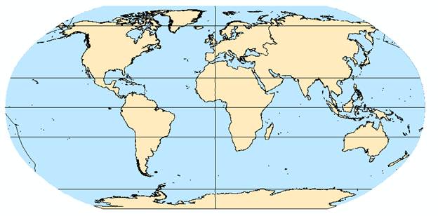
Figure1: World map under Robinson projection provided by ESRI. Robinson minimizes shape and area distortion of world in relation to the equator, such that points within 45 deg range of equator are represented with little distortion. However, the north and south poles are distorted. The center longitude line is the prime meridian.

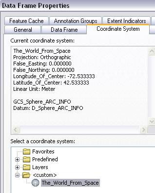
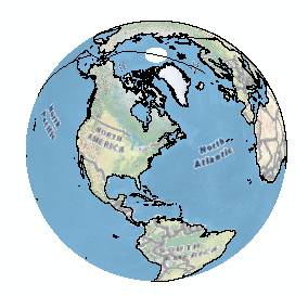
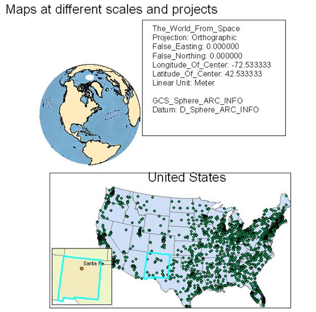
Figure 2: A map of the world using “The_World_From_Space” projection coordinate system provided by ESRI. The predefined projection is spherical which provides a good representation of Earth from a view point from space. This is a good model of the world as a globe shape planet.

Information on map projection was found on ESRI’s website. The ArcGIS Resource Center provided detailed explanation of the features for specific map projections. Here is the link: http://help.arcgis.com/en/arcgisdesktop/10.0/help/index.html#/Robinson/003r0000003z000000/

Mapping the United States

1) A new data frame was generated to include two new layers, states and cities. An important note is that at any time the view can be switched to layout to see the layout which is being constructed (world and U.S maps).

2) A query was built to display state capitals by following this pathway: cities> data properties> query builder> “capitals” = “Y”. Query builder is a tool that shows information of particular interest, in this case, state capitals.

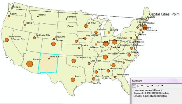
3) City layer properties> symbology tab> show> quantities> proportional symbols defined the capital symbology for population in a range that included three classifications. The population data available for 1990 was used to generate the symbol classification based on size. The legend for the symbol is displayed in the table of contents.

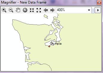
4) Next, the capital names were included to provide an identification using the label feature option. This aided in locating Olympia, WA for a magnification exercise. Olympia was magnified to get a more accurate measurement of the distance from Olympia, WA to Augusta, ME. The distance measured was 4,072 kilometers and after converting units was found to be 2,271 miles. The figure below is an example of Olympia, WA magnified.

5) I changed the coordinate system to be in USA Albers Equal Area projection of United States map, provided by ESRI. The distances between capitals were re-measured following this project and found to be 4,100 km and 2,549 miles. The difference in the distance before and after the application of the projection shows that distance can be distorted. The USA Albers Equal Area projection should reduce the distortion in distance.

6) Next of interest was determining the capital with the largest city and highest elevation. Data was accessed in the “attributes table” and sorted to decrease in values. The capital with the largest population was Phoenix, AZ with 983,403 people. The capital with the highest elevation was Santa Fe, NM at 6989 m.

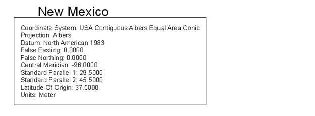
Mapping New Mexico

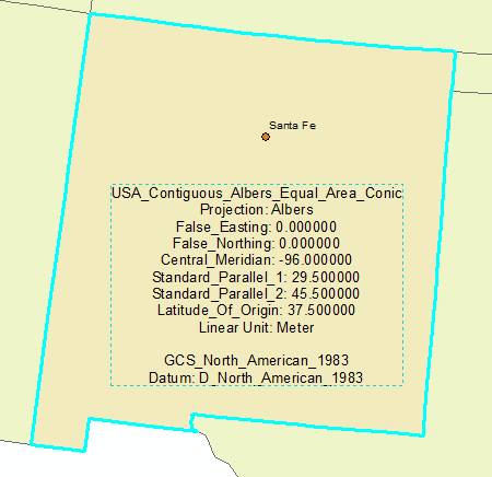
1) The state of New Mexico was selected using the tool and exported from the U.S. map to add another layer named “New Mexico”. The New Mexico layer followed the same coordinate system as the U.S. map in USA Albers Equal Area projection. The output feature class was saved to my geodatabase (G:\GIS\assignment3\map.gdb\new_mexico). The purpose of exporting data is to create another layer within a data frame.

2) I created an additional data frame to allow manipulation of the overall layout. Thus, I had three data frames consisting of “World”, “United States”, and “New Mexico”.

3) Next, I viewed the product in layout form to manipulate the maps, add projection information, and text to designate the maps. There is an interesting scaling affect created during this exercise from Earth>United States> New Mexico. I would like to explore this affect further.

Final Layout: