Rio Puerco Watershed Basin Delineation

In this exercise, we will be delineating a watershed basin just northwest of Bernalillo county called the Rio Puerco watershed. We’ll begin by downloading three files of data, however, they’re interchange files and we need raster data to work with so we need to convert them. Click on ArcToolbox, navigate down to Conversion Tools>To Coverage> Import from E00. Import all three files into ArcGIS and they are automatically converted. You’ll notice that they are not layered one atop the other so we will need to do this ourselves by creating a “Mosaic”. Get back into ArcToolbox then navigate down to Data Management Tools>Raster>Raster Dataset>Mosaic. Use the dropdown menu to add all three files into the “Input Rasters” box, make the first file (e1770) the “Target Raster” and click OK. Your new raster is a mosaic of all three rasters. Uncheck the boxes for E1790 and E1780 in case they are still checked. Now, we want to add some clarity by adding color using the “Symbology” options in the layer properties.

If it’s not already on your toolbar, activate the “Spatial Analyst” tool using the “Customize” option at the top. After it is activated, you’ll need to add the tool itself to your toolbar by using one of the little dropdown bars at the end of the two toolbars you have in ArcGIS.

Next, we’ll begin adjusting our data. In ArcToolbox, navigate down to “Spatial Analyst” tools, and click “Raster Calculator”. We’re going to enter the following function using our keyboard:

Con(IsNull(“mosaic”),FocalStatistics(“mosaic”,NbrRectangle(4,4,”CELL”), “MEAN”), “mosaic”)

The italicized mosaic refers to the unique name that your raster has. Run that calculation and once you get the all clear move on to the next step. A new raster image appears so uncheck the box next to the old one. I relabeled my new raster “no_data”. Next, we’ll fill the spurious pits in our raster. Using the ArcToolbox, navigate to Spatial Analyst>Hydrology>Fill. I renamed my new layer “fill_DEM” so that I know it’s the one that has it’s surface filled in and is ready for hydrologic manipulation. Now, we’re going to begin our hydrologic modeling. First, we want to determine flow direction within this watershed. Open up the ArcToolbox, navigate to Spatial Analyst Tools>Map Algebra>Raster Calculator. Input the following expression (fill_DEM refers to the name I gave my last raster):

FlowDirection(“fill_DEM”)

Next, we’ll create a layer with the flow accumulation by opening up our raster calculator and entering the following formula:

FlowAccumulation(“flow_dir”)

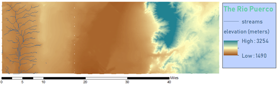
We’re now looking at a raster of accumulated flow to each cell, which as we can recall from class is simply thinking about each cell as holding the amounts that are demarcated on the cells that are flowing into them. Zoom into the left side of the screen so that we are focusing on the Rio Puerco stream network.

Next, we’ll define what we consider to be streams as opposed to creeks or other smaller waterways. Open the Raster Calculator and enter in:

Con("flow_acc">278,1)

This time, however, we’re going to click on “Environments” at the bottom of the calculator window. Click on “Output Coordinates” and use the dropdown menu for “Extent” to find “Same as Display”. This means that the calculator will only focus on processing the area we can see on our screen which in our case is the Rio Puerco mainstem. Removing the other layers from the Table of Contents and leaving behind only the newest raster layer (in my case it’s called streams) we see that if we zoom out the only thing we can see is the Rio Puerco mainstem. Now, we want to convert the raster stream into polyline features. Open Spatial Analyst Tools>Hydrology>Stream to Feature. Use the drop down bars to use your stream raster as the input stream raster and your flow direction raster as the input flow direction raster. Create a new file to use as the Output and click OK. Next, we’ll create a stream network by using the following expression in our calculator:

StreamLink(“streams”, “flow_dir”)

Next, we want to define our outlets by first obtaining the zonal maximum so type the following into the calculator:

ZonalStatistcs(“network”, “VALUE”, “flow_acc”, “MAXIMUM”)

I used the file name “zonalmax” as the output for that expression. After that, we want to define our outlets by using the following expression:

Con("zonalmax"=="flow_acc","network")

I used the file name “outlets” as the output for that expression. Next, we want to use the outlet raster and the flow direction raster to delineate our watershed. Type the following expression into the raster calculator:

Watershed(“flow_dir”, “outlets”)

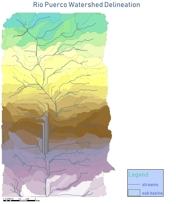
I used the file name “watershed” as my output. We see a conglomeration of colors on our watershed and if you expand the layer properties by clicking the little plus sign next to the layer name you should have roughly 150 sub-basins. I say roughly because this is based upon the cropped area that you chose back when we defined streams so you may have a few more or a few less depending on the extent of your cropping. Now, we are going to delineate our sub-basins by opening the ArcToolbox and navigating to Conversion Tools>From Raster>Raster to Polygon. Your input raster is the one you just created (mine is “watershed”). Uncheck the box for “Simplify polygons” if it is checked (mine was automatically checked), create a name for your polygons (mine is “subbasin_poly”) and click OK.

You have everything you need for your finished product but you may need to change the order of the layers and adjust the Symbology (coloration). I re-organized my layers into the following order from top to bottom because this makes a difference as far as visibility is concerned: streams_poly>subbasin_polys>watershed

I also made the color for the streams darker, chose “hollow” for the color of the sub-basin polygons, and changed the color of the watershed to a gradient featuring less colors.