Appendix
B. GIS Workflow
The
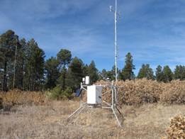
first layer brought in was a simple vector layer displaying the name, location
and agency responsible for each weather station. This was done by creating a
table containing all the relevant information and converting it to a shapefile.
Then tables were created containing each station name, latitude, longitude, and
total evapotranspiration for each 8-day period analyzed. A separate file was
created containing the table for each 8-day period. Each table was converted to
a shapefile. The MODIS raster grid for each corresponding 8-day period was also
brought in. The model below was then run for each period.
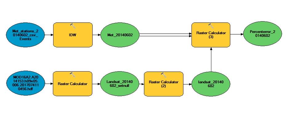
First,
each weather station 8-day evapotranspiration shapefile was converted to a
raster surface using the Inverse-Distance Weighted method, using the ET field
as the Z value.
Next,
erroneous values in the MODIS raster grid were nullified using raster calculator.
In MODIS ET data, fill values of 32761 through 32767 are assigned to erroneous
or missing cells, so cells with values of 32761 and above were assigned NoData. The following expression was used in Raster
Calculator: SetNull(“Input_raster” >= 32761, “Input_raster”), where “Input_raster”
is replaced by the raster layer name. Raster Calculator was used again to fill
cells with nullified values. A cell with NoData was
assigned the average of the four surrounding cells, using the following
expression: Con(IsNull("calculation"),
FocalStatistics("calculation", NbrRectangle(4,4, "CELL"), "MEAN"),
"calculation"), where “calculation” is the name of the
raster layer with nullified erroneous values.
Finally,
the values between the surface raster created using the weather station data
and the “clean” MODIS raster were compared by calculating the percent
difference between the two. The following expression was used: (Abs(“Modis” – “met_station_idw”) /
“met_station_idw”) * 100, where “Modis” is the clean
MODIS raster, and “met_station_idw” is newly
generated surface raster.