Research topics

   - Art of black magic of curve fitting XPS spectra
   - Spectra calibration in XPS
   -  Application of XPS to study electrocatalysts
   - Useful way to compare XPS spectra for multiple samples
   - Systematic study of non-platinum group metal electrocatalysts for oxygen reduction by XPS 

---

Art or black magic of curvefitting XPS spectra

Why talk about something so well known to the surface analysis community as curve fitting high resolution XPS spectra? Two reasons.

First is the skepticism I am running into every time I am showing curve fits of spectra to non-surface analysis communities of scientists. Their reaction is that curve fitting is meaningless as we can curve fit any particular spectrum with infinite number of combinations of peaks of different widths and shapes with the same goodness of fit. So every time I give presentation, which show curve fitting results to people who are not doing it for living, I am talking about physical reasons behindGaussian-Lorentzian shape of peaks, fundamental limits contributing to FWHM and generals rules of accurate reproducible curve fitting.

And the second reason is that even though we all know the rules behind good practices of curve fitting scientific literature is filled with poorly fitted spectra and, therefore, incorrectly interpreted XPS data.

What’s wrong with set of spectra shown on the left. And why spectra on the right represent the “correct” way of curve fitting?

Let’s look at one example from the literature. Three N 1s spectra for three samples (unmodified and heated at two different temperatures) are analyzed.

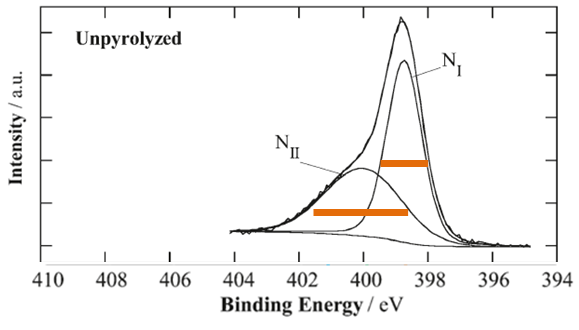
The first sample is unpyrolyzed sample (unmodified)  which is used as a reference. Peak NI is of adequate width for N 1s spectral line. Why, suddenly, peak NII is twice as wide as peak NI?

Heat treatment of sample at 800C introduces changes which are obvious from the spectral shape. Peak NI is at the same position of Binding energy and has the same approximate width. Suddenly peak NII is twice more narrow then it is in unpyrolyzed sample. Peaks NIII and NIV is added to complete a curve fit. Curve fit of this spectrum by itself meets all necessary requiremenets of a good curve-fit in which main three peaks are of approximately the same FWHM. So why there is no peak NIII in unpyrolyzed sample? If one makes peak NII in unpyrolyzed sample of adequate width (being the same as in sample at 800 C), then a third peak NIII must be created to complete a curve fit in the unpyrolyzed sample as well.

At temperature 900 peak NI becomes twice as wide as it is in unpyrolyzed  sample. And peak NII becomes three times more narrow then in unpyrolyzed sample. And, my “intelligent” guess that authors make conclusion on significant decrease of species contributing to binding energy of peak NII from 800 to 900C.

This type of curve fit is exactly why there is so much reservations against use of curve fitting of spectra for quantitative evaluations of changes in chemistries.

And still itt is very easy to do an accurate reproducible curve fit if you remember a few things.

1. Fundamental processes contributing into width of the peak used for curve fitting N 1s, in this case, are the same for all peaks used, i.e. natural width of incident X-ray line,  thermal broadening, pass energy of the analyzer, lifetime of the electron hole, etc. From a reference sample with just one type of N, O or metal, for example, analyzed at your particular instrument it is easy to find what it the adequate width for particular line of the element. ALL peaks within this element should have +/- 0.2 eV the same FWHM. 

2. One of the basis of adequate interpretation of changes introduced by any type of modification isidentification of peaks in unmodified sample. Once the spectra for reference sample are curve fitted, position in BE and FWHM have to be constrained to +/- 0.2 eV each. This curve fit can be then copied into a curve fit of spectra from all other samples in the series. If the set of peaks present in unmodified (reference) sample is not sufficient to complete a curve fit, new peaks of the same FWHM have to be added.

3. If you don’t have reference sample, any sample in a series can be used as “reference” for curve-fit. Then this curve fit can be propagated to all other samples for accurate within samples comparison of changes. CONSTRAINTS, CONSTRAINTS AND CONSTRAINTS! 

4. Cross-correlations of the elements is key! If you have identified, lets say, C-N=O in N 1s spectrum, there should be peak due to the same type of chemistry in both C 1s and O 1s spectra.

These little things will allow you to be as consistent as possible throughout your sample set and make sound conclusions on chemistry.

It is critical to publish and present high quality XPS data processing of spectra to ensure all the trust this powerful method deserves. Let’s do it!

The trivial task of calibraing XPS spectra

This is a schoolbook task. Everybody dealing with XPS spectra knows that if charge neutralizer is used to compensate for charging effect for not fully conductive samples, that causes spectra to shift to lower BE. In order to correct for that spectra must be calibrated/charge corrected/shifted – whatever the word you’re using to describe this procedure.

Adventitious carbon contamination is a vice but its virtue is that all samples (almost) have it so we can reliably use it for calibrating spectra for lots and lots of materials. Its position is assumed to be 284.8 eV. Put maximum of C 1s spectra to that position and use the same shift for all other spectra from that position for that sample and voila!

But what if carbon is a major part of the material you’re designing or studying? Is it mainly graphitic (284.4 eV), aromatic (284.7 eV), aliphatic (285 eV)? Are there lots of surface oxides causing big secondary shift of C at 285.5 eV? How can you reliably use C as internal standard when you may know nothing about the carbon itself? Putting maximum of a carbon peak at 284.8 eV (assumed to be representative of internal hydrocarbon), how sure are we that we are not calibrating all of the spectra by graphitic or secondary carbon? The difference of 0.4-0.6 eV may not seem significant but we can not claim to being able to resolve peaks as close as 0.2-0.3 eV and accurately identify them at such accuracy of calibration, can we?

If we put Au or Ag reference material (which are available as paints, pens or powders) onto each sample individually, we can see the effect. Figure shows that for bipyridine the difference between using C and Au for calibration is small, being only 0.2 eV.

However, for another sample shown, CoTMPP,  the difference in calibration is 1eV. So if we would’ve used C (and we did) we would incorrectly identified types of Co and N and O present within the sample.

The purpose of surface analysis of most functional advanced materials is to be able to correlate surface chemistry to whatever parameter of performance or of interest. In this particular example state of N is of critical importance in understanding what is the structure of active site in the electrocatalysts. Pyrrolic N and pyridinic N are among the suspected species responsible for oxygen reduction. And, coincidentally, the difference in BE between N in pyridine and pyrrole environment is … Yes, you guessed it right – 1 eV – exactly as we have found the difference between calibrating by Au and by C. So, if we would’ve used C, we would’ve found that majority of N is in pyrrolic state and if we would’ve used Au, we would conclude that it is pyridinic that is the main type of N.

Now wonder that out of 35+ manuscripts reviewed, N speciation in pyropolymers or fuel coals as determined by XPS shows huge spread of reported values for all major types of N.

Is it because all of them used carbon as internal standard for calibrating their spectra?

I think you know the answer…

---

Trends in applications of XPS to electrocatalysts:

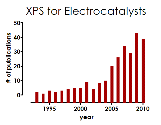Review on "Application of XPS to study electrocatalysts for fuel cells" published in Journal of Power Sources by A. Wieckowski group

---

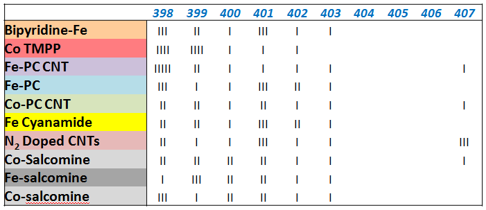
Useful way to compare XPS spectra for multiple samples

- building a quantitative "histogram" of amount of species in relative % as a function of Binding energy. Each bar in a plot corresponds to ~10%.

---

Systematic study of non-platinum group metal electrocatalysts for oxygen reduction by XPS 

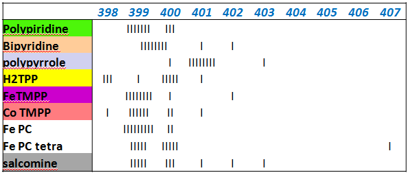
Different routes for Me-N-C containing electrocatalysts exists. We have studied precursors and electrocatalysts obtained by following procedures: 1. Transition metal-containing macrocyclic compounds such as cobalt and iron phthalocyanines and porphyrins heat treated at various temperatures. 2. Derived from nitrogen-containing polymers (polyacrylnitrile, polypyrrole, etc.) and/or low-molecular-weight precursors (e.g. cyanamide , doped with transition metal salts. 3. Activation” of carbonaceous materials in the presence of nitrogen precursors and transition metals as well.
Hypothesis:

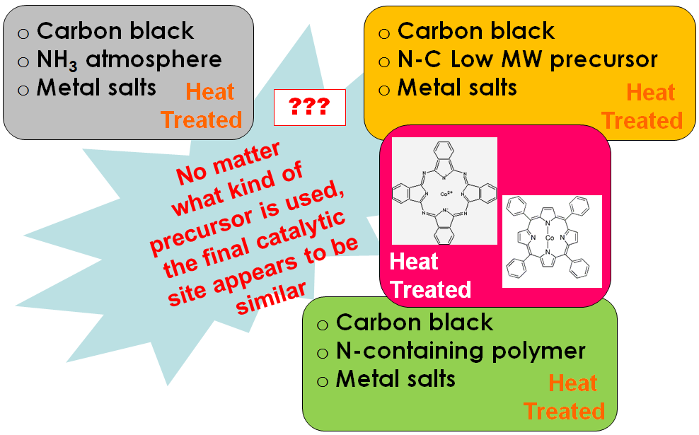
XPS analysis of precursors and electrocatalysts confirmed that from any type of starting mixture end up in very similar type of material with the same types of N, Me and C moieties. Distribution of moieties is responsible for electrocatalytic activity.
As a result of "cooking the recipe" in various ways, one comes from large distribution of N species to much smaller variation of species: