CE547 Index > Experiments in Projection
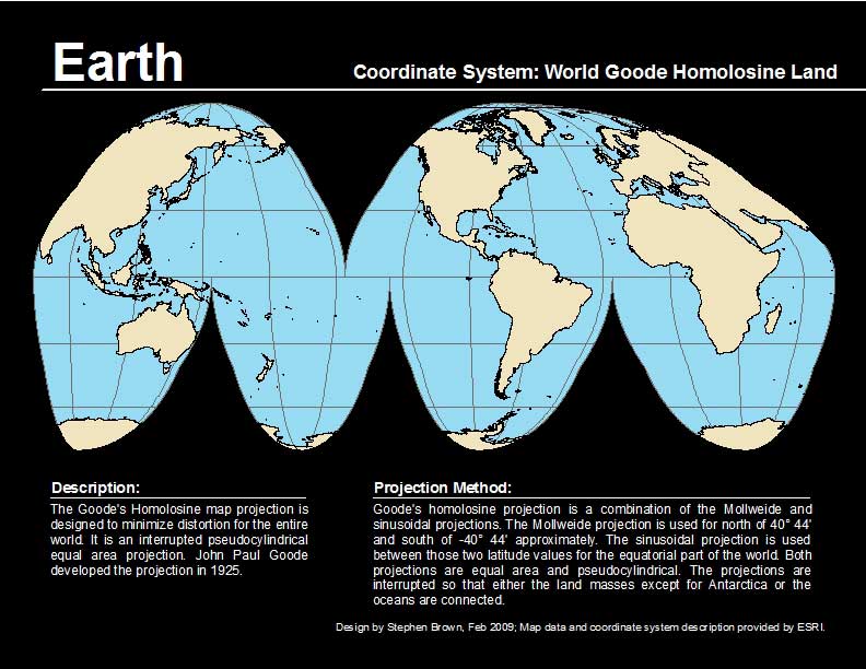
Steps for World map:
- Open ArcMap, Add new layers (World Continents and Map Background) from the ESRI template geodatabase.
- In Map Backgroud layer, changed fill and outline to blue symbolizing water.
- In World Continents layer, changed fill to tan symbolizing land.
- In Data Frame, changed projection to Goode's Homolosine Land. This is a projection designed to reduce distortion for the entire world. Goode's method of splitting the map results in an equal area projection. Additional benefit is that it looks cool.
- In layout I added title and supplemental text.
- Exported map to JPEG and PDF, click image to see PDF.
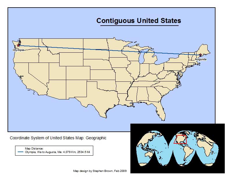
Steps for USA map #1:
- Open ArcMap, Add new layers (US Cities and US States in Data Frame 1 and World Continents and Map Background in Data Frame 2) from the ESRI template geodatabase.
- In Data Frame 1, entered "CAPITAL" = 'Y' AND "CITY_NAME" = 'Augusta' OR "CITY_NAME" = 'Olympia' in Definition Query to isolate specific cities for analysis and changed symbol to red star.
- In Data Frame 2, changed parameters to match previous world map.
- In Layout Mode, drew lines connecting cities for distance measurement, then using measure tool, measured distance in kilometers and converted to feet.
- In Layout Mode, I added extend rectangle, title and supplemental text.
- Exported map to JPEG and PDF, click image to see PDF.
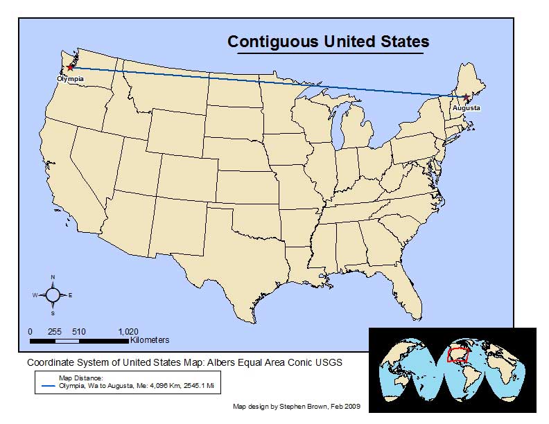
Steps for USA map #2:
- Using existing un-projected map, I projected the US Data Frame to Albers Equal Area Conic.
- In Layout Mode, re-drew lines connecting cities for distance measurement, then using measure tool, measured distance in kilometers and converted to feet.
- In Layout Mode, I resized USA map and updated distances.
- Exported map to JPEG and PDF, click image to see PDF.
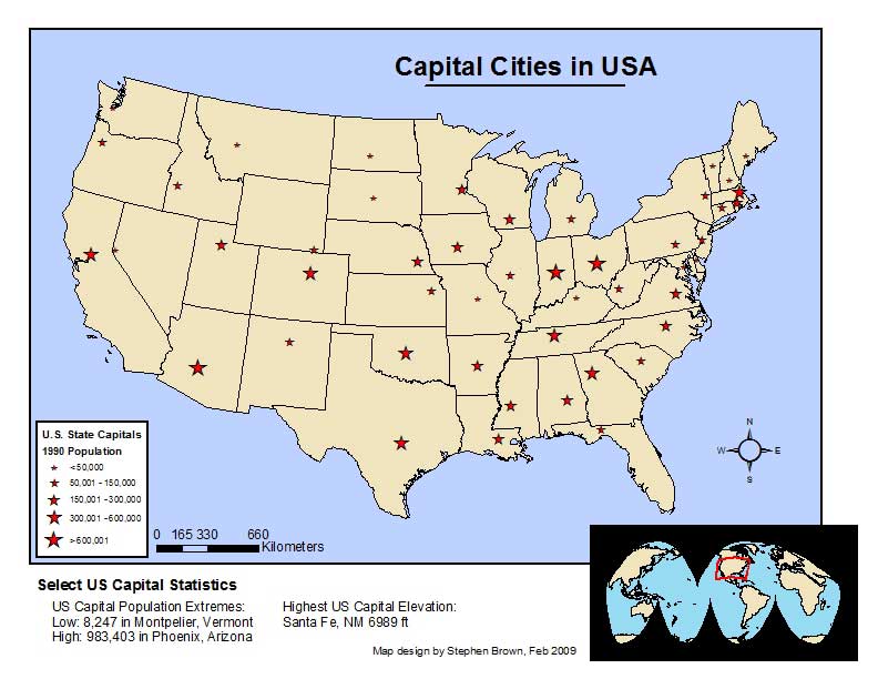
Steps for USA map #3:
- Using existing projected map, I changed the Definition Query to "CAPITAL" = 'Y' isolating state capitals.
- While in the layer properties, I changed the symbology of the cities to show stars of increasing size for differences in city size.
- Investigating the Attribute table for the cities I sorted the POP1990 field in ascending order to find the city with lowest and highed population. Similar process on the elevation field revealed the city with highest elevation.
- In Layout Mode, I added a legend for all cities and typed details regarding the lowest and highest populations and highest elevation.
- Exported map to JPEG and PDF, click image to see PDF.
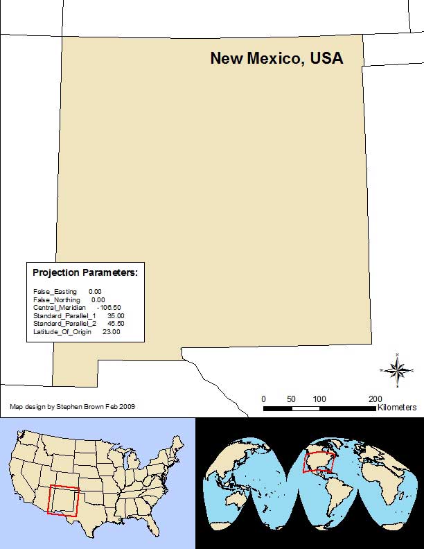
Steps for New Mexico map:
- Using existing projected map, I added another Data Frame for the New Mexico data and proceeded to add two identical US States layers.
- In first states layer, I entered "STATE_NAME" = 'New Mexico' in Selection>Select by Attributes to isolate New Mexico.
- Right clicking on States layer, I selected Data>Export and saved the layer as nmgeo.shp
- In the second states layer I changed the symbology to show just the state outlines to show states around New Mexico.
- In both of the states layers I projected the layers to Albers Equal Area Conic using Data Managment Tools>Projections and Transformations>Feature>Project
- The Project tool saved the output from the New Mexico map to nmgeo_Project.shp and the second states layer to states_Project.shp.
- Loading the saved layers back in to the Data Frame, I changed the Central Meridian to -106.5, centering the map view on Albuquerque, NM.
- In Layout Mode, I added a text box with Projection Parameters and added extent rectangles to US and World inset maps.
- Exported map to JPEG and PDF, click image to see PDF.