Defining the Jemez Watershed and Stream Discharge Patterns using ArcGIS

By Betsy Shafer

6 May, 2011

Introduction

The Jemez River is a tributary to the Rio Grande and supplies it with surface water due to snow melt and precipitation events. Thus identifying tributary subbasins is important in estimating the amount of discharge entering the Rio Grande. Understanding climate dynamics is also important as it varies annually and seasonally which impacts discharge in head water streams. Objectives for this project include 1) delineate Jemez watershed using the hydrology tool ; 2) compare the hydrographs at three USGS stream gage sites for a time period of 1981 to 2003; 3) use time animation to present hydrograph during the selected time period. The East Fork Jemez River is my research site so watershed delineation and data management is of primary interest.

Methods

The Digital Elevation Model for the Jemez watershed area was downloaded on the USGS seamless server website (http://seamless.usgs.gov/). The DEM was spatially analyzed using hydrologic modeling tools in ArcMap to determine stream network and delineation of the Jemez subbasin. Historical discharge data from 1981 to 2003 was obtained at State of New Mexico USGS Water Resource Division for three stream gage sites (http://nm.water.usgs.gov/). Spatial and temporal data was added to watershed map in ArcMap.

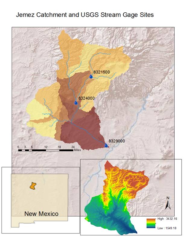
Figure 1: Elevation map Jemez catchment and delineated catchment with USGS Stream Gages. Created in ArcMap.

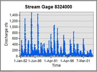
Figure2: Hydrographs arranged from high to low elevation for stream gage sites from 1981 to 2003.

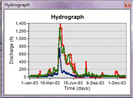
Figure 3: Annual hydrograph comparison for each gage site in 1983. Stream reach is represented by color: blue is upper, green is middle, and red is lower.

Results

Comparison between USGS stream gage sites shows variability in discharge from 1981 to 2003 (Figure 2). The hydrograph for the high elevation site shows interannual variable with extreme discharge years. The middle reach hydrograph show interannual variability as well but also shows higher baseflow as would be expected being a higher order stream. The lower reach is below Canyon Dam thus flow is regulated, however, flow variability among years is still present. Overall, Figure 3 shows interannual variation in stream discharge between sites and and within a site. Furthermore, the annual hydrograph for year 1983 shown in Figure 3 was selected due to it being a high discharge year. Differences in discharge are noticeable in respect to time, the upper reach stream flow peaking first, and amount, the lower reach discharge is greatly more.

Conclusions

The ability to graph stream discharge data over time is advantageous when merging temporal and spatial data and displaying as x,y data in ArcMap. Additionally, hydrologic modeling quantitatively measures stream features as well as the influence of surrounding area. The Jemez system is dynamically driven by climate factors such as snow and precipitation in which data can be used for future work to model stream discharge in response to climate change. Other factors include soil properties, geomorphology, and riparian vegetation which can be displayed spatially in ArcMap as well as surfaces. Future work will focus more specifically on stream metabolism and how the mentioned factors influence primary and consumer productivity over time. I predict that stream metabolism will be greater in high elevations where slope gradients are low, riparian coverage is less, and discharge is lower. Ultimately, stream metabolism can be displayed spatially as a surface.

References

Ormsby, Napoleon, Burke, Groessl, Bowden. 2010. Getting to know ArcGIS Desktop 10. ESRI Press: Redlands, CA.

United States Geological Survey. (Updated 12/28/2010). Seamless Data Warehouse. Retrieved 4/15/2011. http://seamless.usgs.gov/

United States Geological Survey. (Updated 2/3/2011). New Mexico Water Science Center. Retrieved 4/15/2011. http://nm.water.usgs.gov/