New Mexico Primary Care
Physician Accessibility Models
Preliminary Analysis with R - 2002
Data
Larry Spear,
UNM (10/15/2018)
This preliminary analysis using R
will eventually compare all the results from the generalized two-step methods
and the one-step models. Various distance decay method; exponential, power, Gaussian,
and DGR power have been used. Several analytical techniques will be employed including;
exploratory data analysis (graphics), ANOVA and related diagnostics, Moran’s I
test for spatial autocorrelation, and spatial oriented ANOVA. Only the results
and a brief discussion are presented here. A more comprehensive version
including the data and R code will be prepared later using Jupyter
Notebook. Also, an ArcGIS Online Story Map with a more in-depth discussion of
results will be developed in the future.
The following Group or Item names
have been used to designate the individual methods:
2SEE - Two Step Hybrid Zonal,
Exponential Function
2SEG - Two
Step Hybrid Zonal, Gaussian Function
2SEP - Two
Step Hybrid Zonal, Std. Power Function
2SED - Two
Step Hybrid Zonal, DGR Power Function
1SED - One
Step Hybrid Zonal, DGR Power Function
1SEE - One
Step Hybrid Zonal, Exponential Function
1SEG - One
Step Hybrid Zonal, Gaussian Function
1SEP - One
Step Hybrid Zonal, Std. Power Function
Two-Step Methods Compared with
One-Step (DGR) Method
This preliminary analysis using R
will be based on a comparison of the generalized two-step methods using
exponential, power, and Gaussian distance decay with the one-step method using
the DGR power distance decay method. Additional comparisons of two-step methods
with the other one-step methods (exponential, power, and Gaussian distance
decay) will also be presented later after the analysis procedures have first
been tested and refined here.
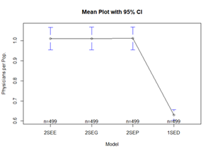
Summary Statistics
- table shows the resulting means, standard deviations, minimum and maximum
values (physicians per 1000 population) for the two-step and one-step (DGR)
accessibility models (ACC Methods):
Group count mean
sd
min max
<ord> <int>
<dbl> <dbl> <dbl>
<dbl>
1 2SEE 499 0.988 0.892 0.0000290 7.36
2 2SEG 499 0.990 1.10 0 10.3
3 2SEP 499 1.00 0.772 0.227 5.79
4 1SED 499 0.630 0.305 0.0437 2.74
Note: The one-step method (1SED) with the
DGR power decay has both a lower mean (0.630) and less variance (0.305) than
all the two-step methods. There are two other important mean values to be
considered. The overall statewide mean derived by dividing the state population
estimate (1,874,591) for 2002 by the estimated number of primary care
physicians in 2002 (1,167) is 0.62235. The county-based service area (COSVAR)
mean is 0.437665. The closest mean values to the statewide mean is derived by
using the one-step methods (small difference primarily due to round off).
Boxplots, Histograms – and related plots are useful for
visualizing the differences between the one-step (DGR and the two-step methods:
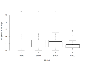
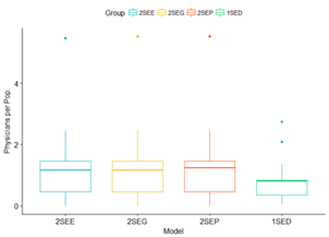
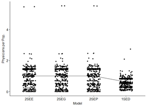
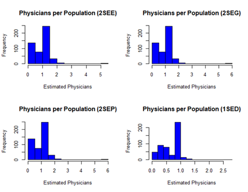
Note: These plots clearly indicate that
there may be a significant difference in the two-step method results compared
with the one-step method. The median values, interquartile ranges, and outliers
(maximum values) are very different. It is also apparent from the histograms
that neither of the resulting distributions appear to be normally distributed.
ANOVA (one-way) – test and related results
are shown below. The Null Hypothesis (H0) is that the
means from the various methods are the same. The Alternative Hypothesis
(Ha) is that at least one of the methods is not equal to the others.
Df Sum Sq
Mean Sq F value Pr(>F)
Group 3
54 17.998 53.75 <2e-16 ***
Residuals 1992
667 0.335
---
Signif. codes: 0 ‘***’ 0.001 ‘**’ 0.01 ‘*’ 0.05 ‘.’ 0.1 ‘ ’ 1
Tukey multiple comparisons of
means
95% family-wise confidence level
Fit: aov(formula = Phys_per_P ~ Group, data = data_test1_df)
$`Group`
diff lwr upr p adj
2SEG-2SEE 0.0000242485 -0.09416672 0.09421522 1.0000000
2SEP-2SEE 0.0006913828 -0.09349959 0.09488236 0.9999976
1SED-2SEE -0.3795959920 -0.47378697 -0.28540502 0.0000000
2SEP-2SEG 0.0006671343 -0.09352384 0.09485811 0.9999978
1SED-2SEG -0.3796202405 -0.47381121 -0.28542927 0.0000000
1SED-2SEP -0.3802873747 -0.47447835 -0.28609640 0.0000000
Levene's Test for
Homogeneity of Variance (center = median)
Df F value Pr(>F)
group 3 59.671 < 2.2e-16 ***
1992
---
Signif. codes: 0 ‘***’ 0.001 ‘**’ 0.01 ‘*’ 0.05 ‘.’ 0.1 ‘ ’ 1
One-way analysis of means (not
assuming equal variances)
data: Phys_per_P and
Group
F = 103.65, num df = 3.0, denom df = 1032.2, p-value < 2.2e-16
Pairwise comparisons using t
tests with non-pooled SD
data: data_test1_df$Phys_per_P and
data_test1_df$Group
2SEE
2SEG 2SEP
2SEG 1 -
-
2SEP 1 1
-
1SED <2e-16 <2e-16 <2e-16
P value adjustment method: BH
Shapiro-Wilk normality test
data: aov_residuals
W = 0.85362, p-value <
2.2e-16
Kruskal-Wallis rank sum test
data: Phys_per_P by Group
Kruskal-Wallis chi-squared =
170.93, df = 3, p-value < 2.2e-16
Note: - As the p-value (<2e-16 ***) is so
small the ANOVA test indicates that the Null Hypothesis (H0)
can be rejected in favor of the Alternative Hypothesis (Ha).
There appears to be a significant difference between at least one of the
methods means and the others. However, there are three important assumptions or
requirements that should be considered when applying ANOVA. 1) The data are
independent and obtained randomly from the population; 2) The data are normally
distributed; and 3) The data have common variances. All these assumptions have
not been met here and these results should be interpreted with caution. These
results are not independent or obtained from a random experiment. There is
evidence of more than moderate spatial autocorrelation (see Moran’s I test).
The previous histograms show that the data are not normally distributed. The
summary statistics show a lack of common variances. Regardless, it is important
to present these results using standard ANOVA and related diagnostic
techniques. If necessary, routine measures such as data transformations can be
subsequently employed. Also, research is underway to eventually conduct a
spatial ANOVA test to see if there is any noticeable change in the results.
The
additional routine diagnostic tests confirm the initial observations and
standard ANOVA results. The Tukey multiple comparison of means indicates that
the one-step method always has a low p-value (0.0) when compared with any of the two-step
methods. The Leven’s test for homogeneity of variance also has a low p-value (2.2e-16 ***) that
suggests that the variances are not common across methods. The pair-wise t test
with no assumption of equal variance also indicates that the one-step method is
significantly different from the two-step methods, p-values (<2e-16). The
Shapiro-Wilk normality test p-value (< 2.2e-16) also indicates a lack of normality. The
Kruskal-Wallis rank sum test (non-parametric) which can be used when ANOVA
assumptions are not met does not change the outcome, p-value (< 2.2e-16) confirming
the Null Hypothesis (H0) can be rejected in favor of
the Alternative Hypothesis (Ha). Additional
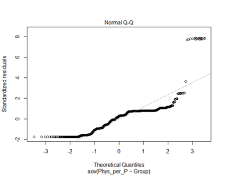
confirmation of concern for caution in interpreting the ANOVA results is
apparent by reviewing the Normal QQ plot of standardized residuals that should
be mostly normally distributed. The residuals deviate considerable from a
straight line, confirming a lack of desired normality.
Moran’s I – global test for spatial
autocorrelation using a queen’s case neighbors list and row standardization
results for each method are shown below:
Neighbour list object:
Queen’s case
Number of regions: 499
Number of nonzero links: 2960
Percentage nonzero weights:
1.18875
Average number of links:
5.931864
Weights style: W
Weights constants summary:
n
nn S0 S1
S2
W 499 249001 499 185.3664
2095.07
moran.range(Results.lw)
[1] -0.7214727 1.0623680
Moran I test under
randomisation
data: Results_Pop_Phys_spdf$Phys_2SEE
weights: Results.lw
Moran I statistic standard
deviate = 17.861, p-value <
2.2e-16
alternative hypothesis: greater
sample estimates:
Moran I statistic Expectation Variance
0.4786685352
-0.0020080321 0.0007242812
Moran I test under
randomisation
data: Results_Pop_Phys_spdf$Phys_2SEG
weights: Results.lw
Moran I statistic standard
deviate = 17.715, p-value <
2.2e-16
alternative hypothesis: greater
sample estimates:
Moran I statistic Expectation Variance
0.4746291857
-0.0020080321 0.0007239152
Moran I test under
randomisation
data: Results_Pop_Phys_spdf$Phys_2SEP
weights: Results.lw
Moran I statistic standard
deviate = 17.825, p-value <
2.2e-16
alternative hypothesis: greater
sample estimates:
Moran I statistic Expectation Variance
0.4776201197
-0.0020080321 0.0007239826
Moran I test under
randomisation
data: Results_Pop_Phys_spdf$Phys_1SED
weights: Results.lw
Moran I statistic standard
deviate = 21.084, p-value <
2.2e-16
alternative hypothesis: greater
sample estimates:
Moran I statistic Expectation Variance
0.5673121641 -0.0020080321 0.0007291042
Note: There is significant spatial
autocorrelation for the one-step and all the two-step methods (similar Moran’s
I statistics, very low p-values, and large standard deviates). These results
indicate strong clustering and it is extremely unlikely (less than 1%) that
these clustered patterns could be the results of random chance. The one-step
method is perhaps even more clustered (a larger Moran’s I statistic) than the
two-step methods. This lack of independence is a violation of a major standard
ANOVA assumption. A not that widely used or well documented alternative test
method that can take into consideration non-independence or spatial
autocorrelation is spatial ANOVA. This method is currently being researched and
results will be available soon.
Spatial ANOVA (one-way) – currently
being prepared!
Note:
Two-Step Exponential Method Compared
with One-Step Exponential Method
currently
being prepared!
Two-Step Power Method Compared with
One-Step Power Method
currently
being prepared!
Two-Step Gaussian Method Compared
with One-Step Gaussian Method
currently
being prepared!
Summary of Results
currently
being prepared!
Larry Spear
Sr. Research Scientist (Ret.)
Division of Government Research
University of New Mexico