© The University of New Mexico, Albuquerque, NM 87131, (505) 277-0111

This assignment will show you the first step of many hydrologic analyses, basin delineation.
a) Download data: The files for this project are called ArcInfo Interchange files. An interchange file contains all coverage information and appropriate INFO table information in a fixed-length ASCII format.
You will need these three files: E177.E00 E178.E00 E179.E00 They are available by ftp from the cegis account. Currently they are in a different format from rgis.unm.edu.
b) Import E00: Activate the ArcToolbox to convert the interchange files into coverages. Click on the red tool box icon. From Conversion Tools > To Coverage > Import from E00

c) Adding toolbar: Add the three coverage files into your new map document. Click Customize > Extensions & check Spatial Analyst for later use of special tools in ArcToolbox. You can also add the Spatial Analyst toolbar from Customize > Toolbars. Dock the toolbar to a more convenient location on your screen.

d) Mosaic rasters: Since three files are not continuous, we need to use the mosaic tool from the ArcToolbox to make them a continuous surface. Click on data Management Tools > Raster > Raster Dataset > Mosaic. The input raster files are the three downloaded ones. The target raster is the first raster on the list of input raster files. The new raster 177 now gets the lowest elevation from raster 178 and the highest elevation from raster 179.

e) Colorize Raster: Now change the color ramp of the adjoined raster from the Symbology tab in the Layer Properties. Remove raster layers 178 & 179 from the map document. Right click on Properties of raster 177, from the General tab, change the name of raster 177 to a more descriptive name.


f) Fill spurious pits in raster: You need to fill the surface by using the ArcToolbox tool: Spatial Analyst > Hydrology > Fill.

Now you have a DEM that is prepared for hydrologic modeling.
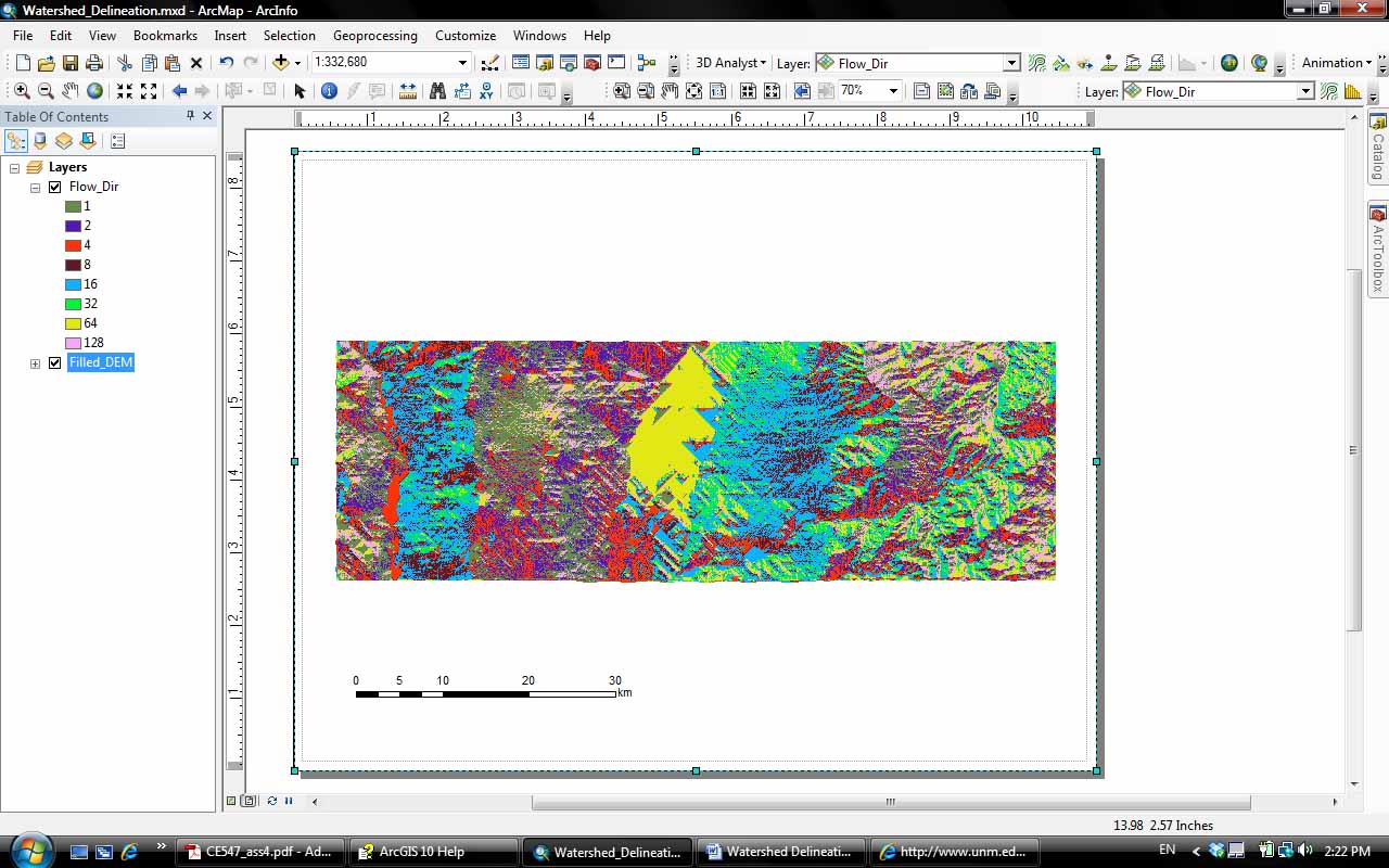
a) Flow direction:
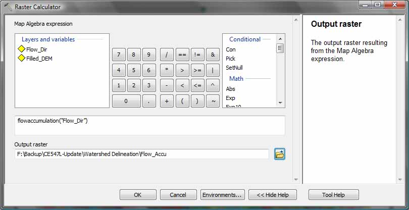
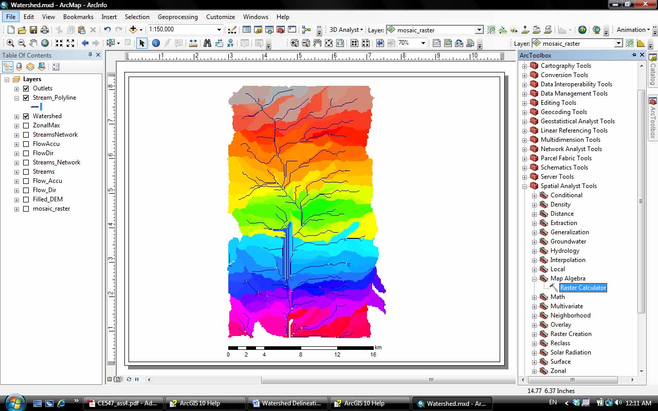
From the ArcToolbox, use Spatial Analyst Tools > Map Algebra > Raster
calculator to open the Raster Calculator window.
Raster Calculator expression: FlowDirection(“Filled_DEM”). The
“Filled_DEM” is the name of the raster file I use. You may have given it
a different name than mine. (Note that using the Raster Calculator for
this assignment may give you some additional modeling ideas.)

Or ArcToolbox: Spatial Analyst > Hydrology > Flow Direction

There are eight valid output directions relating to the eight adjacent cells into which flow could travel. This approach is commonly referred to as an eight-direction (D8) flow model.
b) Flow Accumulation:
Raster calculator expression: FlowAccumulation("Flow_Dir"). Again my
“Flow_Dir” may have a different name than yours.
Or ArcToolbox:
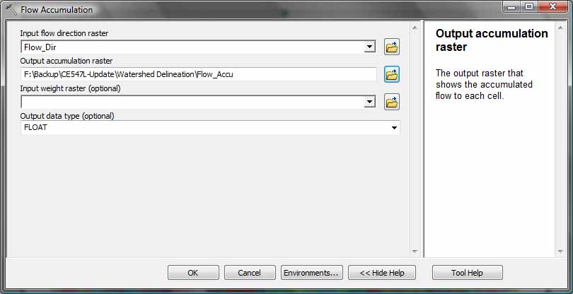
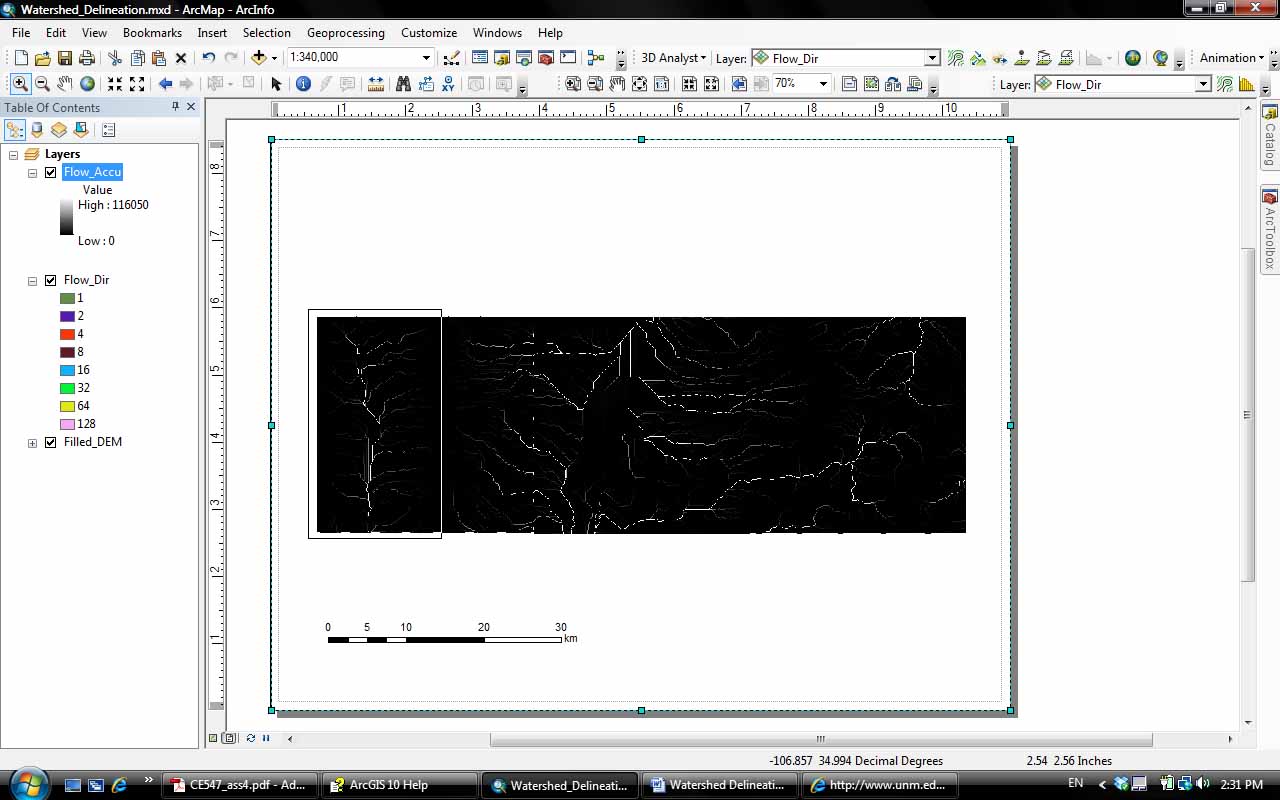
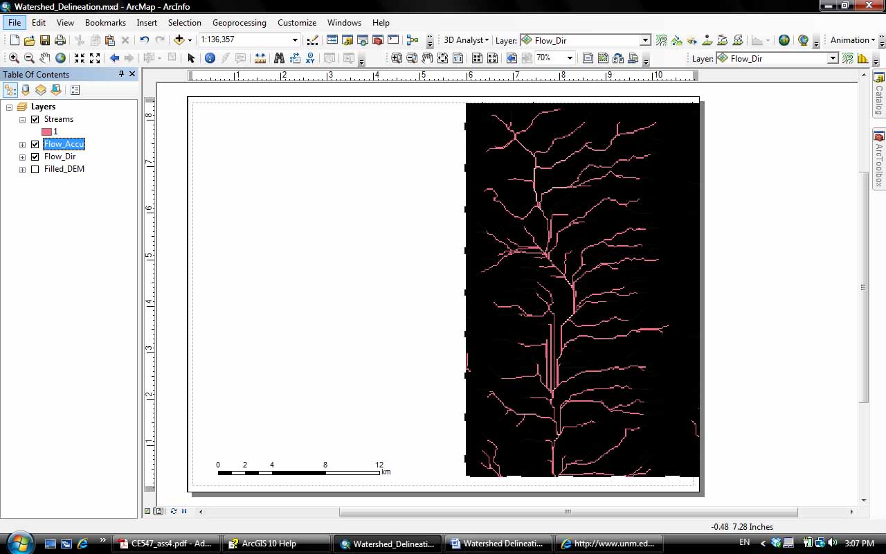
The result of Flow Accumulation is a raster of accumulated flow to each cell, as determined by accumulating the weight for all cells that flow into each downslope cell. Zoom to the box on the left of the screen since the stream network (The Rio Puerco) is more continuous in this area.
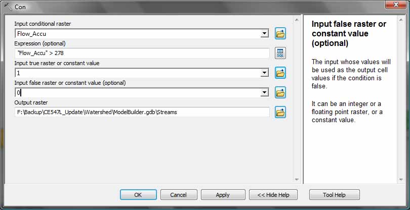
c) Stream definition:
Each cell has an approximate size of 60 m x 60 m and the drainage area
threshold is defined to be greater than 1 km2. Therefore, in 1km2 there
are about 278 cells. All cells with more than 278 cells flowing into them
will be defined as streams.
The raster calculator expression is: Con("Flow_Accu">278,1)
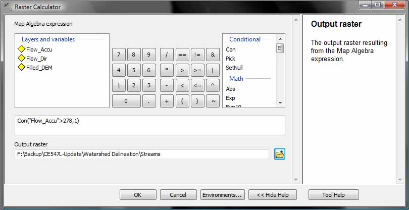
If you select the 'Environments...' button at the bottom of the Raster Calculator dialogue box, you are able to adjust things like the Analysis Extent (to the Display) so that you're not performing the analysis on the entire grid. This can be very useful if you have a huge grid and only need analyses for a small area.
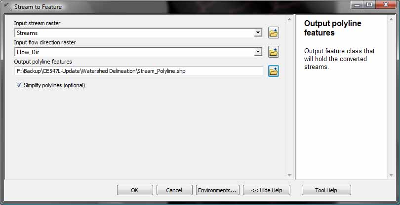
Convert the raster stream into polyline features based on the
vectorization of rasters.
Arctoolbox: Spatial Analyst > Hydrology > Stream to Feature

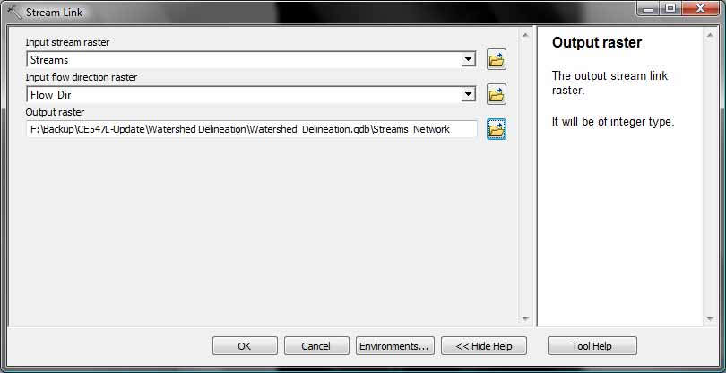
d) Stream network creation:
Raster calculator expression: StreamLink("Streams","Flow_Dir")
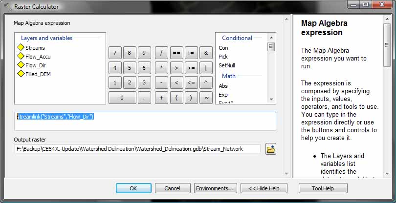
Or ArcToolbox: Spatial Analyst > Hydrology > Stream Link

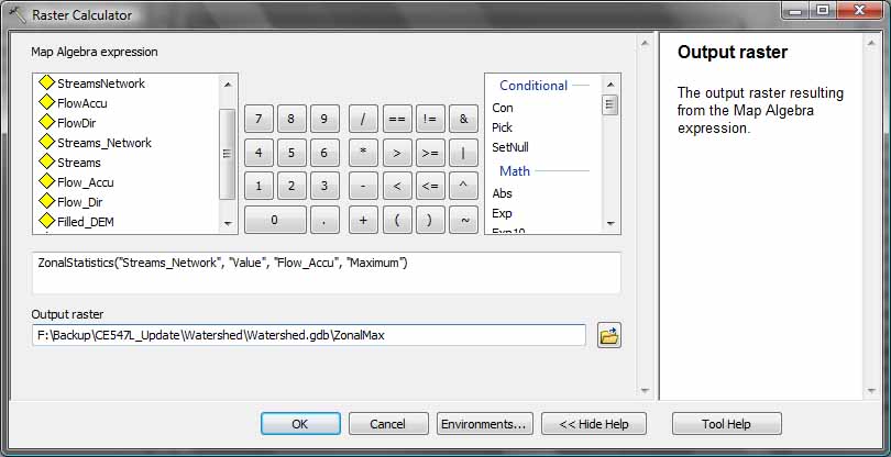
e) Defining outlets:
Raster calculator expression: ZonalStatistics("Streams_Network", "Value",
"Flow_Accu", "Maximum"). You need to have a space after each comma in the
command line. Otherwise, you’ll get an error message. This function is
similar to the zonalmax expression in ArcGIS 9 which no longer works for
ArcGIS 10. Remember to utilize ArcGIS Help to get more
information about individual tools and functions.
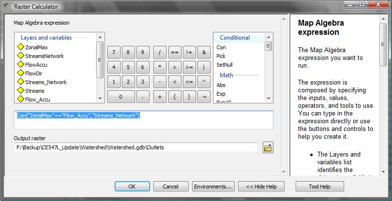
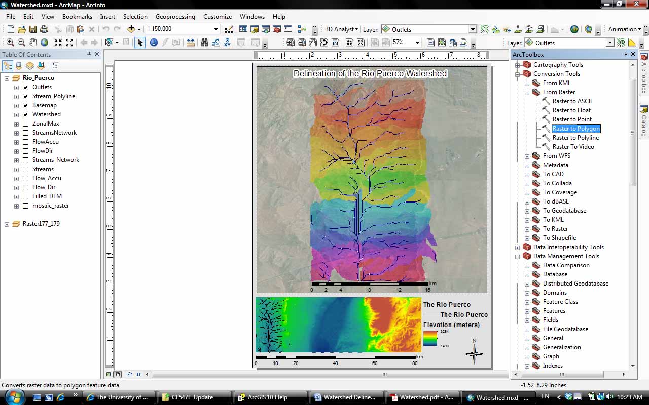
Raster calculator expression: Con("ZonalMax"=="Flow_Accu","Streams_Network"). Do not leave any space between the two equal signs or you’ll get an error message. If you are familiar with ArcGIS 9, you may notice that the Conditional function is capitalized in ArcGIS 10.
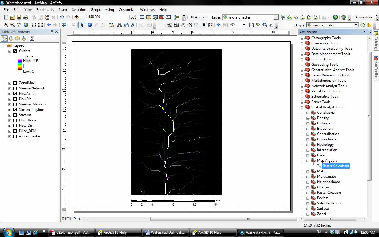
The screen capture below shows the colored outlets with the stream polyline features.
f) Delineate watersheds:
Now let’s use the outlets and flow direction rasters to delineate the
watershed.
Raster Calculator expression: Watershed("Flow_Dir", "Outlets").
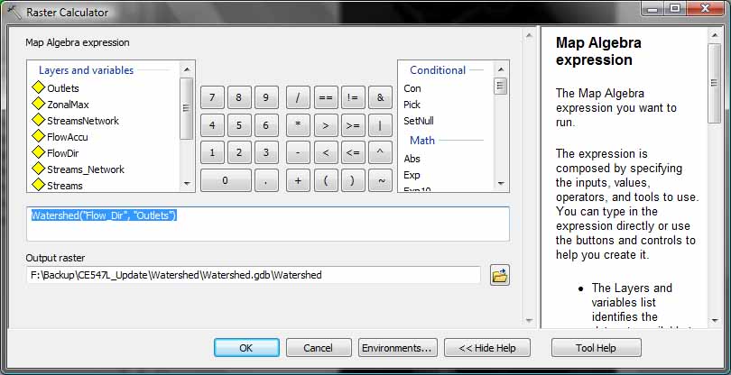
From the Properties of the newly created Watershed raster, there are 153
sub-basins based on the stream threshold we defined previously.
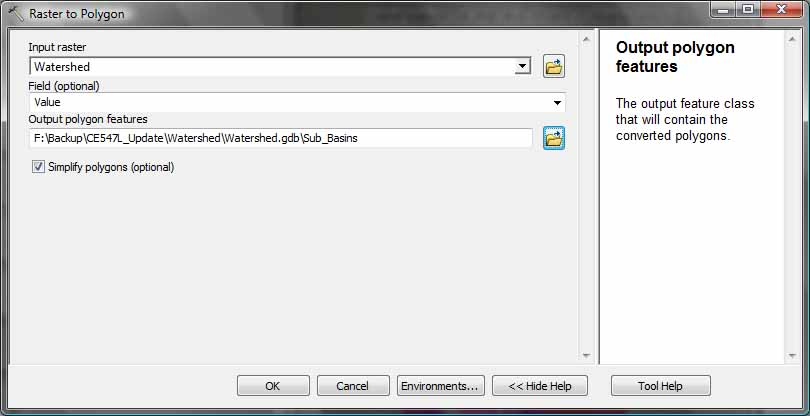
Export the sub-basins of the watershed into polygons:
From ArcToolbox: Conversion Tools > From Raster > Raster to Polygon
g) Review files:
Go to your Geodatabase in Catalog menu along the right side of your
screen. You will be surprised to see how many new files you have created
for this assignment.
Final Map Layout:
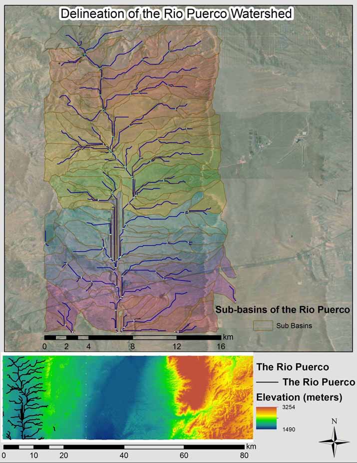
Export finished map showing your basin delineation and add to your website.
|
Layer name |
Description |
Expression for Raster
Calculator |
|
Raster1 |
flow direction |
FlowDirection("elev") |
|
Raster2 |
flow accumulation |
FlowAccumulation("Raster1") |
|
For the remaining calculations, choose a
smaller analysis extent such as the Rio Puerco area.
More specific instructions follow. |
||
|
Raster3 |
Streams (with > 1 km2
drainage area) |
Con("Raster2" > 278,1) |
|
Raster4 |
Stream links |
streamlink("Raster3", "Raster1") |
|
Raster5 |
|
ZonalStatistics("Raster4", "Raster2", "max") |
|
Raster6 |
outlets |
Con(("Raster5" = = "Raster2", "Raster4") |
|
Raster7 |
watersheds |
Watershed("Raster1", "Raster6") |
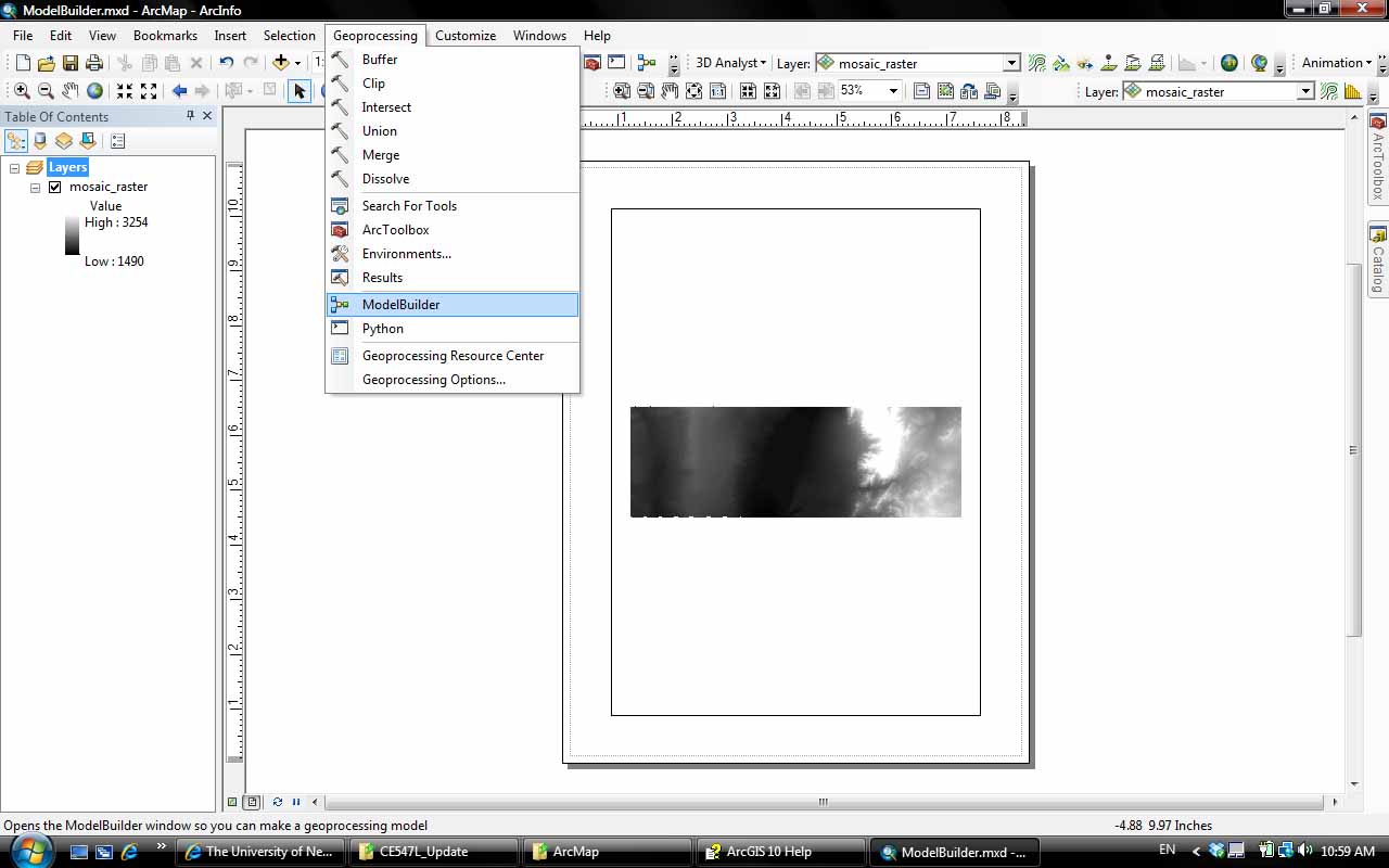
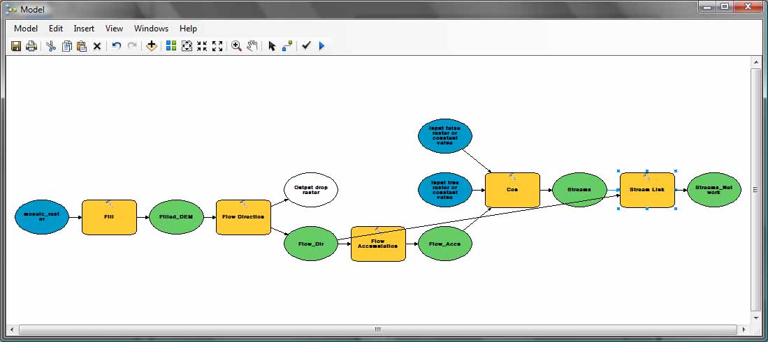
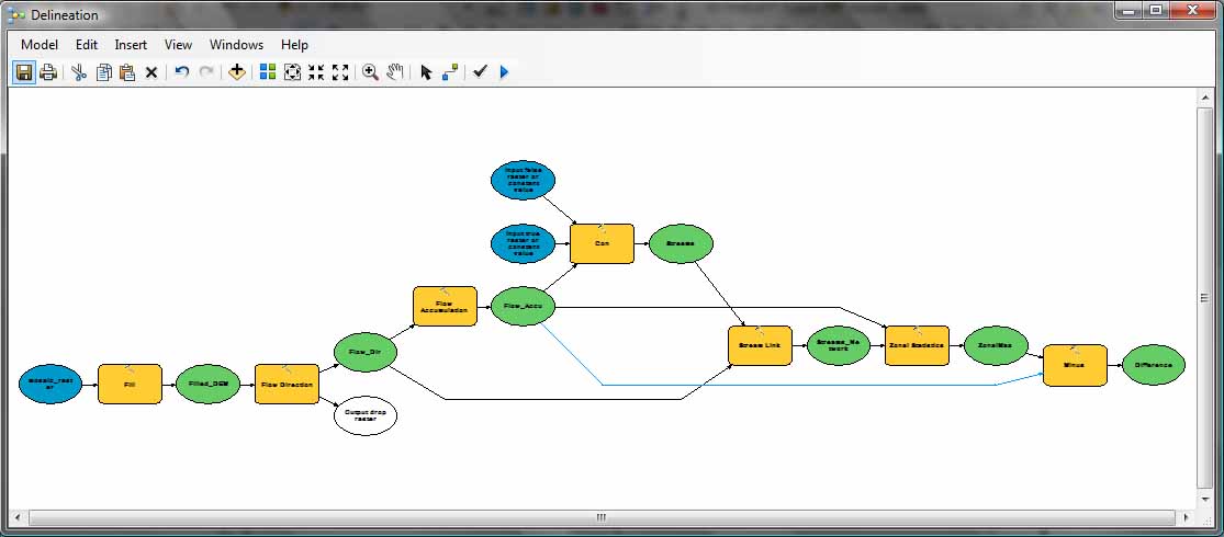
a) Start ModelBuilder: Geoprocessing > ModelBuilder
After you added the three rasters and merged them, you can start the model builder.
The sequence of steps is similar to all of the work you just did before
making the final map layout. However, once you have created your model,
you can use it for different inputs and it automates the calculations for
you. You can save your model as one comprehensive tool in your ArcToolbox
which includes all steps to delineate a watershed.
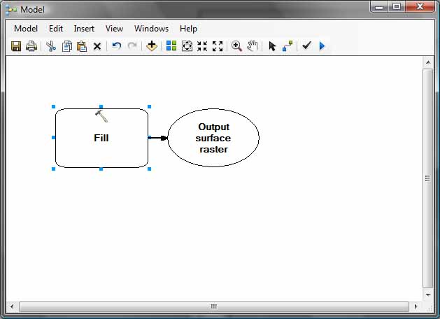
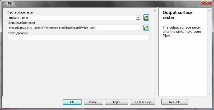
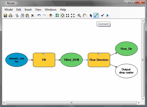
b) Fill DEM:
From the ArcToolbox, Hydrology > Fill. Drag the Fill tool into the Model
Builder window. Double click on the Fill tool, it opens up a window for
your input and output rasters.
c) Flow Direction:
Drag in the Flow Direction tool. Use the connect icon on the Model
Builder window to connect Filled_DEM to the Flow Direction tool.
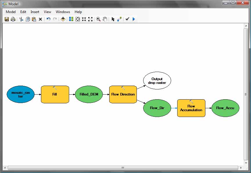
d) Flow Accumulation:
Drag the Flow Accumulation tool in. Use the connect icon to connect
Flow_Dir with the Flow Accumulation tool.
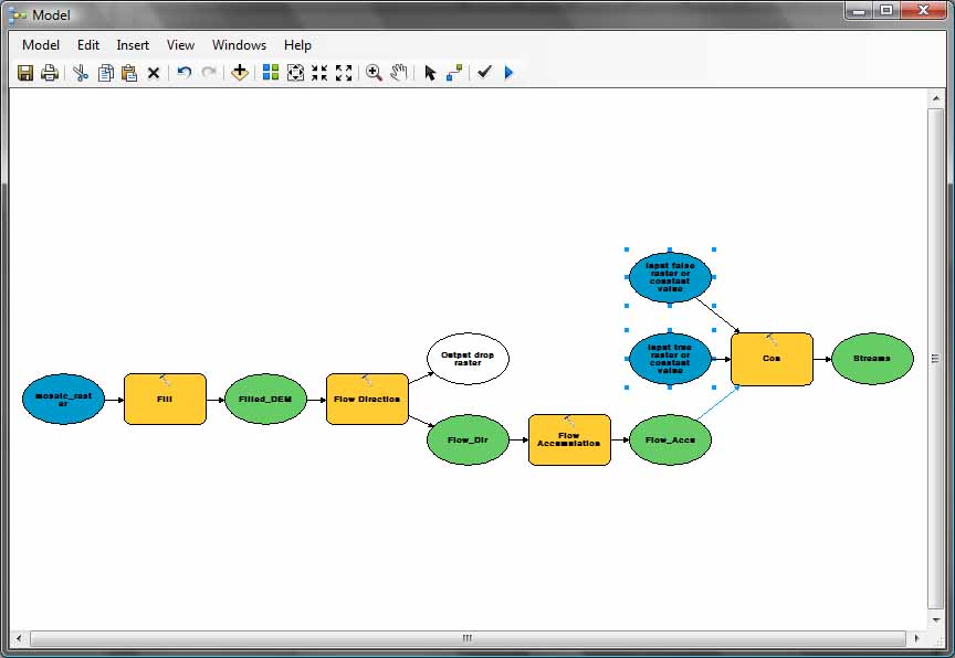
e) Stream definition:
From ArcToolbox, use Spatial Analyst Tools > Conditional > Con. Drag the
Con tool into the model window. Connect Flow_Accu with the Con tool.
Follow the Con tool window for inputs.
f) Stream Network:
Drag the Stream Link tool into the model window. Connect Streams with the
Stream Link tool.
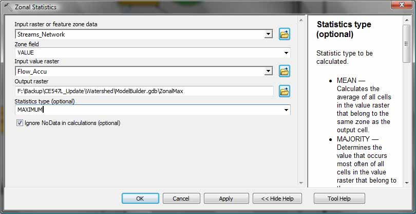
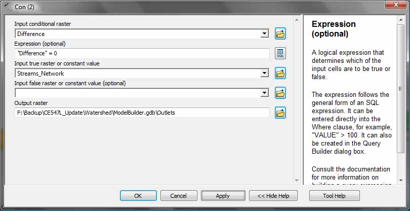
g) Outlets:
From the ArcToolbox, go to Spatial Analyst > Zonal > Zonal Statistics.
Drag the tool into the model window.
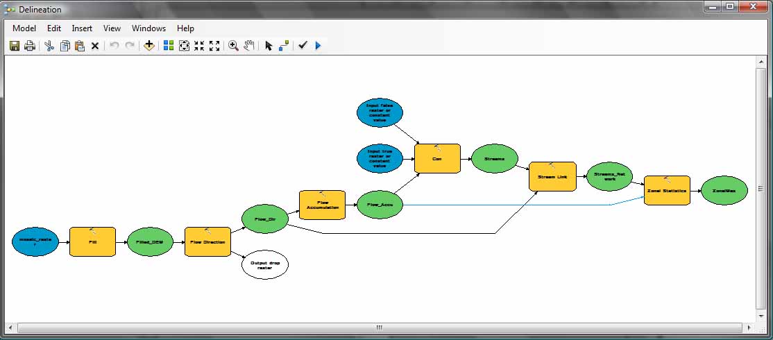
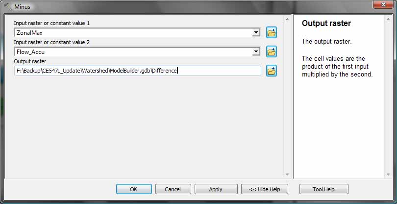
From the ArcToolbox, use 3D Analyst > Raster Math > Minus. Drag the minus tool into the model window.
From the ArcToolbox, use Spatial Analyst > Conditional > Con. Drag the Con tool into the model window.
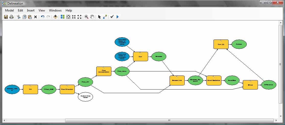
h) Watershed:
From the ArcToolbox, use Spatial Analyst > Hydrology > Watershed. Drag
the Watershed tool into the model window.
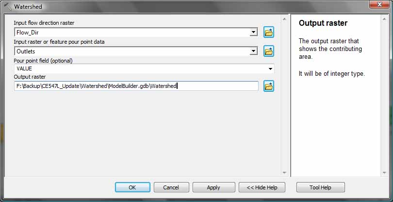
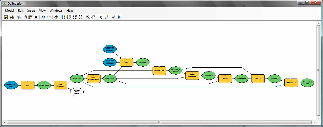
i) Run Model:
Click on Model > Run to test your model. You can save this model as
Delineation Tool in the ArcToolbox.