© The University of New Mexico, Albuquerque, NM 87131, (505) 277-0111

This exercise is intended to introduce you to soils data from the STATSGO soils coverage as well as land use data. The STATSGO Users Guide is available online http://www.fsl.orst.edu/pnwerc/wrb/metadata/soils/statsgo.pdf. In addition, you will learn about joining and relating tables and about some geoprocessing commands.
For this assignment you will again use the headwaters of the Pecos basin. You’ll use the STATSGO coverage for New Mexico. You’ll “clip” (using the ArcToolbox) a portion of STATSGO to conform to the watershed boundaries of pecoshuc (which you worked with in the previous assignment). Tabular data on the soil properties are provided by the Info tables Mapunit, Comp, and Layer, which are held separately from the soil coverages in the Info directory. Finally, the exercise looks at the land use in the study region and the coinciding characteristics between land use and soil type.
a) Download data: Assignment6.gdb.zip is available from the CEGIS account. All the data you need for this assignment is already included in the gdb. If you were beginning this analysis for yourself, the shapefiles and tables for the soils region would need to be imported to your gdb. In case you're up for the challenge, the raw data is available from the STATSGO website: http://www.soils.usda.gov/survey/geography/statsgo/
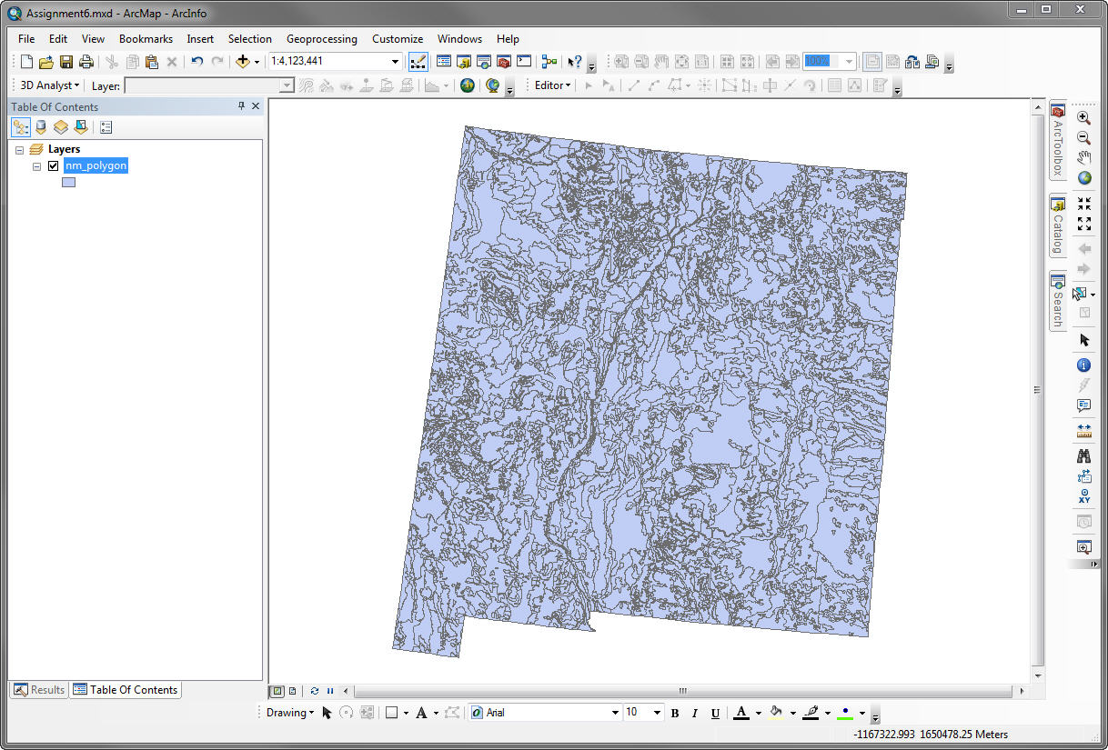
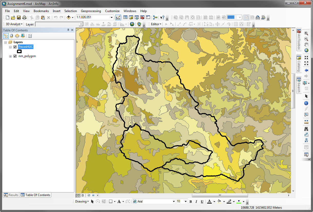
b) Load soil data: Add the nm_polygon layer from Assignment6.gdb. There are 2083 features in the New Mexico STATSGO soils layer.
Clearly this is an immense data base, but the large size of its polygons makes it suitable for analysis of fairly large areas which contain several STATSGO polygons. There is another database called SSURGO, still under development by US Dept of Agriculture, which details soil polygons at the component level rather than at the map unit level. SSURGO currently has limited coverage in New Mexico. You can find out more about SSURGO data on the NRCS website (http://soils.usda.gov/survey/geography/ssurgo/) .
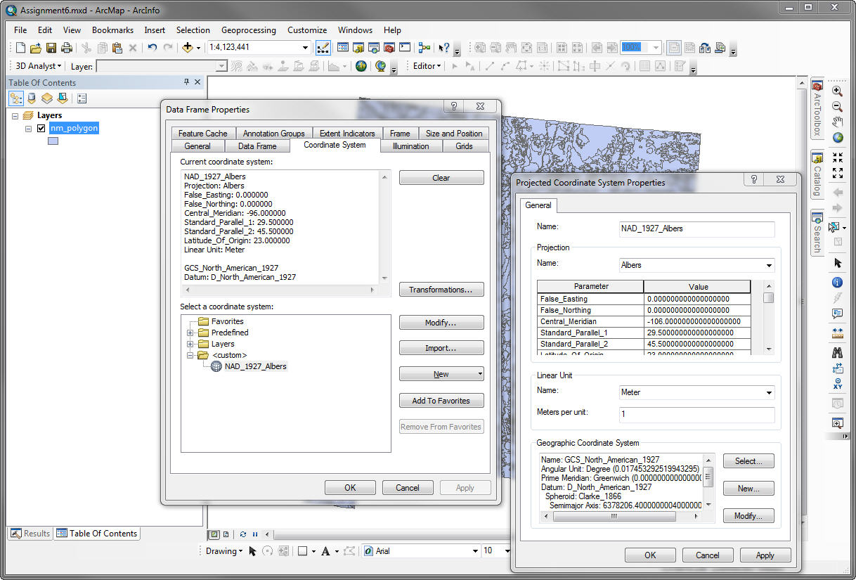
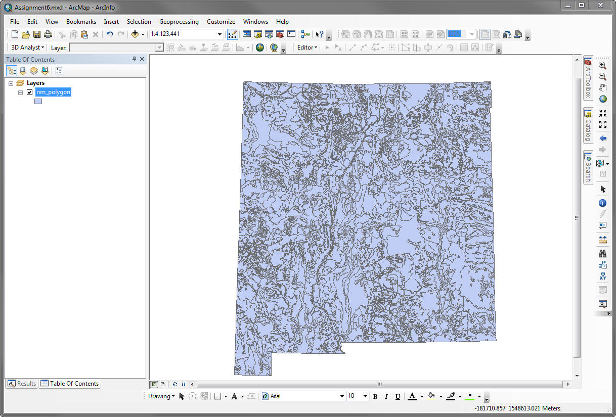
c) Change map alignment: Notice how the New Mexico is tilted to the right.
 .
.
This tile is controlled by the Central_Meridian setting under Data Frame Properties > Coordinate System. Navigate into Data Frame Properties and change the Central Meridian from -96 to -106. This moves the center of the layer 10 degrees to the west making the state stand up straight.
d) Update symbology: Change the symbology so that your data frame has more meaning.
e) Add PecosHUC: Next, you need to add the headwaters of the pecos watershed, PecosHUC. Change the symbology of PecosHUC so that the polygon is hollow. Note that some of the polygons of STATSGO correspond with watershed boundaries (i.e. rock outcroppings along edges, polygon following the river valley, etc).
f) Extract soils for Pecos headwaters: Next, we’ll use the ArcToolbox to clip the boundaries of STATSGO to that of our watershed. ArcToolbox> Analysis Tools > Extract > Clip. Follow the dialogue boxes as shown below. Click ‘Show Help’ to learn more.
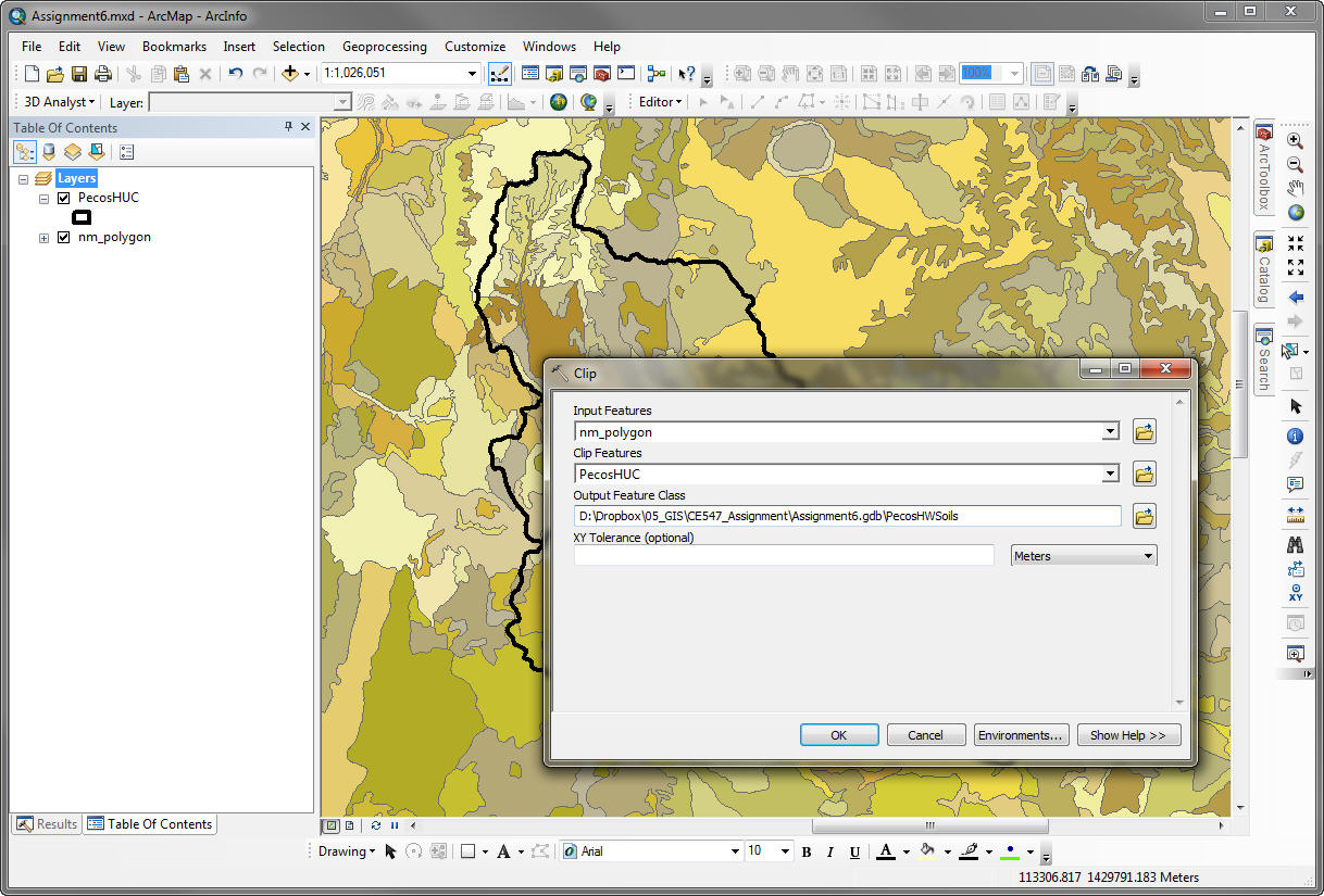
Now, you’ll have 86 records in your table instead of 2084.
g) Add tables to map: Next, we’ll add the tables you need to really get the information that STATSGO offers. Drag comp, layer, and mapunit tables from your geodatabase into the Table of Contents. You may want to go back to the STATSGO website and view the Users Guide to find more about the tables and the information available in each table.
Once the tables have been added, the Table of
Contents window will automatically switch to the Source tab
![]() . Take
a look at all of the tables to get an idea of the information they
contain. (Right
click for the context menu which will allow you to open the table.) The
attribute table for your clipped STATSGO layer is of limited use
without the other tables. So our next step will be to provide the appropriate joins and relates
to get the information that we want.
. Take
a look at all of the tables to get an idea of the information they
contain. (Right
click for the context menu which will allow you to open the table.) The
attribute table for your clipped STATSGO layer is of limited use
without the other tables. So our next step will be to provide the appropriate joins and relates
to get the information that we want.
Some of the fields in the comp table are as follows:
Muid - the mapunit id number e.g. NM963
Muname - the descriptive name of the map unit
Seqnum - a number from 1 to 21 that identifies which soil component of this
map unit is being described.
Compname - the name of this soil component.
Comppct - the percentage of the map unit occupied by this component.
Slopel - lower limit of surface slopes for this component
Slopeh - upper limit of surface slopes for this component
Surftex - USDA soil texture type (C = clay, S = sand, Si = Silt, L = loam, F
= fine, G = gravel, and combinations of these include CL for clay
loam, SL for Sandy Loam, etc)
Hydrgrp - hydrologic soil group (A = sandy, free draining soil, D = clayey,
poorly drained soils, B and C are intermediate soil groups.)
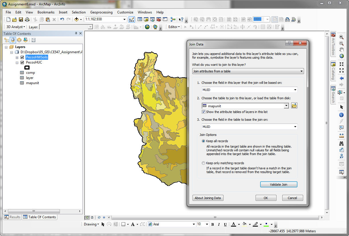
h) Joining Tables: The mapunit table will at least provide a name corresponding with each mapunit. To join information from the mapunit table to the attribute table of PecosHWSoil (or whatever you named your clipped soil layer), right click the layer name for the context menu and select Joins and Relates > Join. . .
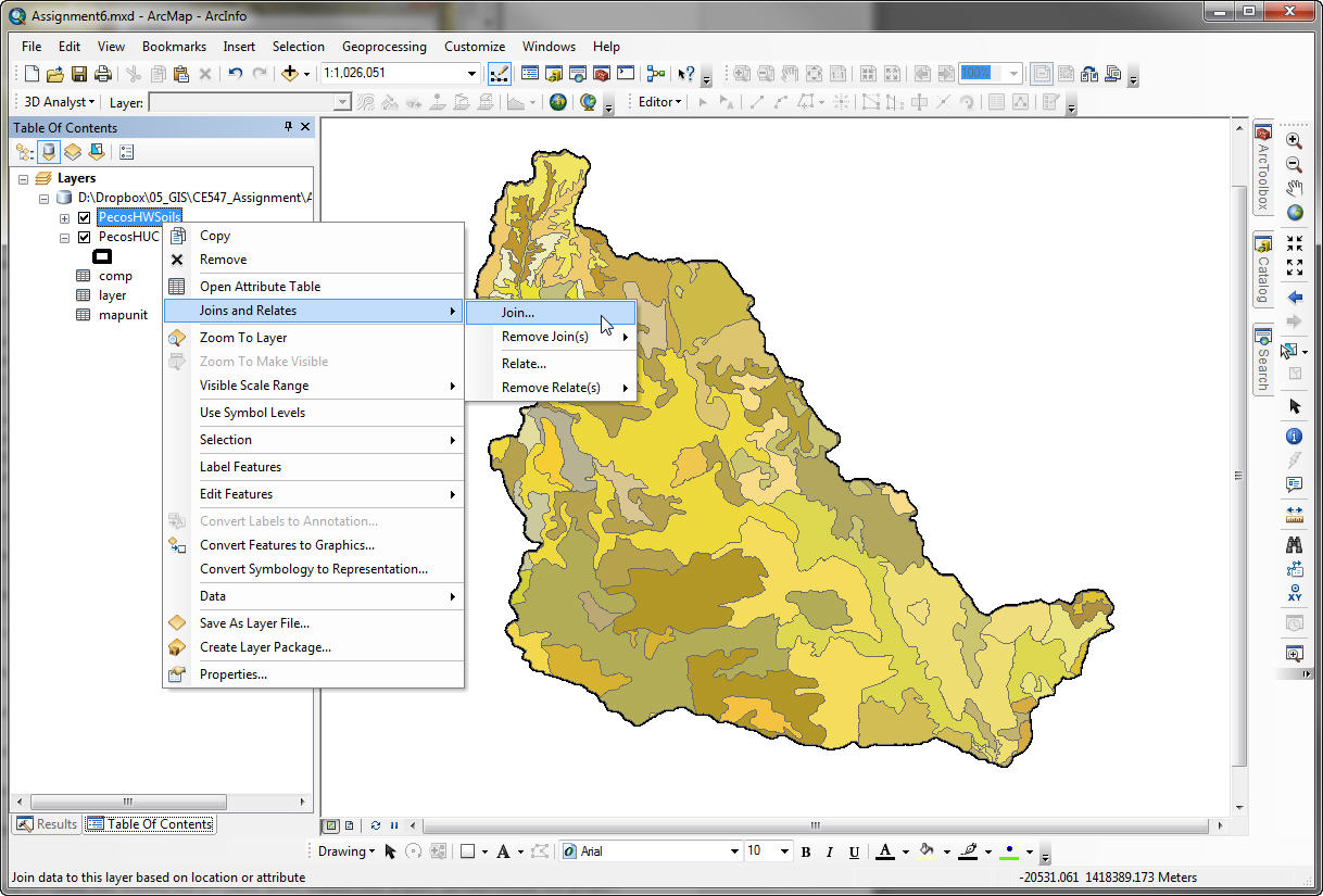
This many-to-one join is simple as shown by the dialogue boxes below. Click the ‘About joining data’ button to learn more.
After completing the join, note the new fields in your attribute table. There is still a lot more information that can be gleaned from this database if we relate the attribute table to the comp and layer tables. Each mapunit is made up of a number of components. If we relate the soils layer to the comp table we will have a one-to-many relate where one record in the mapunit table is related to many records in the component table.
a) Spatial Averaging Soil Properties: Using the table joins from the previous steps, the average properties of soils in a particular map unit can be determined using a weighted average of the component properties where the weights are equal to the percentages contained in the comppct field. For example, map unit NM572 contains soils with two surface textures: L (loam) for component 1 and GR-L (gravel loam) for component 2. The percentage of the total area in the map unit occupied by these components is 50% and 50%, respectively.
To be turned in:
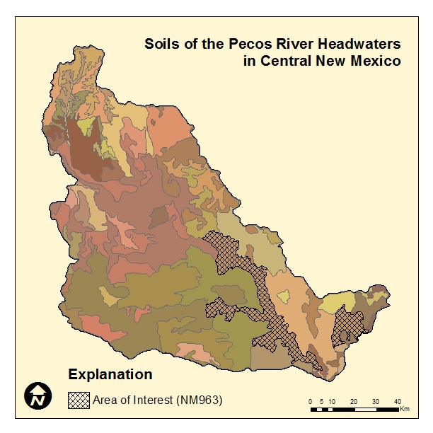
b) Export map: Export a finished map showing map unit NM963 and add to your website.
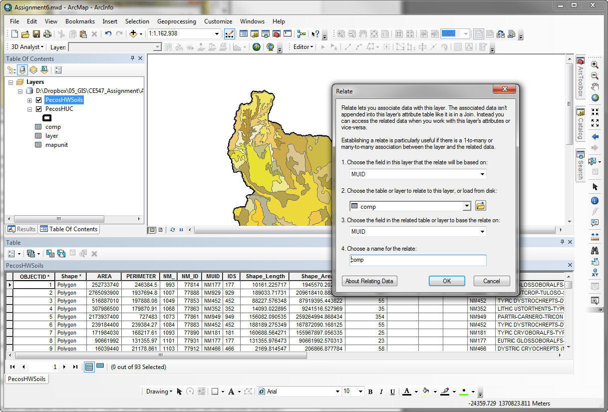
c) Relate comp and layer tables: Next you should relate the component table (comp) with the layer table (layer).
The component properties describe the soil as a whole. Soils are usually divided into soil horizons beginning at the surface, and each horizon or layer has different physical properties. These are contained in the Layer table.
In the Table of Contents window, click on Source tab so that you can see your tables. Right click the Layer table to access the properties. In the Table Properties, with the Fields tab, note that you can choose which fields to show. Click off all the field names except the following: Muid, Seqnum, Layernum, Laydepl, Laydeph, Awcl and Awch (Awch is located near the end of the table).
These properties represent:
Muid and Seqnum - the mapunit and component identification numbers
defined in the component table.
Layernum - an integer between 1 and 6 that describes the number of layers,
with layer number 1 being the uppermost layer.
Laydepl - the depth of the top of the layer in inches.
Laydeph - the depth of the bottom of the layer in inches.
Awcl - a lower limit on the estimated water holding capacity in inches of
water per inch depth of soil (e.g. a value of 0.16 in/in means that
16 per cent of the soil volume is void space that could be occupied
by water).
Awch - an upper limit on the estimate water holding capacity.
Relate the Layer and Comp tables together. Use the same procedure as before as you used to relate the mapunit and comp tables.
The mapunit table should now be related to the
comp table and the comp table to the layer table. Click on Muid
NM963 in the mapunit table and once it is highlighted, you should
see the corresponding components and layers highlighted. If you
don’t, you’ll need to select Options in the bottom right hand corner
of the table, click Related Tables and the name you gave the
relationship.
d) Vertically Integrating Soil Properties:
Soil Depth: The total depth of the soil layer is equal to the value of laydeph for its deepest component. For example, for map unit NM963, Component 1 has depth 0 - 9 inches for layer 1, 9 - 18 inches for layer 2, and 18-22 inches for layer 3 so the total depth is 22 inches for this component.
The average depth can be found as:
Average Depth = Sum over all components of (comppct/100) * component depth
Available Water Capacity: In the layer table, the Available Water Capacity is given in dimensionless units of inches of water / inch of soil. In soil water analysis, we need to know the Water Holding Capacity of the soil, that is, the total depth of water that the soil could store within its whole vertical profile. To calculate this, we first find an average value of available water capacity for each soil layer by averaging the low and high values for that layer, (awcl + awch)/2, multiply the result by the layer thickness (laydeph - laydepl), and sum over all the layers:
Water Holding Capacity of each Component = sum over its layers of (awcl + awch)/2 * (laydeph - laydepl)
This gives a result in inches of water. For example, for mapunit NM963, Component 1 is a Regnier clay loam having three layers, with awcl = 0.18, 0.14, and 0.00, respectively and awch = 0.20, 0.16, and 0.00. The average awc = (0.18 + 0.20)/2 = 0.19 for layer 1; (0.14+0.16)/2 = 0.15 for layer 2 and 0.00 for layer 3. Layer 1 is 9 inches thick so its water holding capacity = 0.19 * 9 = 1.71 inches, and similarly, Layer 2 being 18 - 9 = 9 inches thick, has a water holding capacity of 9 * 0.15 = 1.35 inches of water. Layer 3 has no water holding capacity. The total water holding capacity of the Regnier Clay Loam component soil is 1.71 + 1.35 = 3.06 inches of water, whose storage is distributed throughout the pore spaces of the top 18 inches of soil.
The average value of the water holding capacity of the soils in the NM963 map unit is found as a weighted average of the values in each component using the comppct percentages as weights:
Average Water Holding Capacity for the Map Unit = Sum over all its components of (comppct/100) * Water Holding Capacity of each Component
Computing the average water holding capacity for a map unit is a fairly involved calculation so it is probably best to transfer the data to Excel and do the calculations there. If you right click on the table layer, you can go to the Data > Export Menu and export the selected records of that Table into a new Table. If you choose the .dbf in the Export dialog you will produce a dBase file that can be read directly by Excel. Exporting and transferring the required records from the comp and layer tables to a spreadsheet may save you time in transcribing the data values manually.
To be turned in:
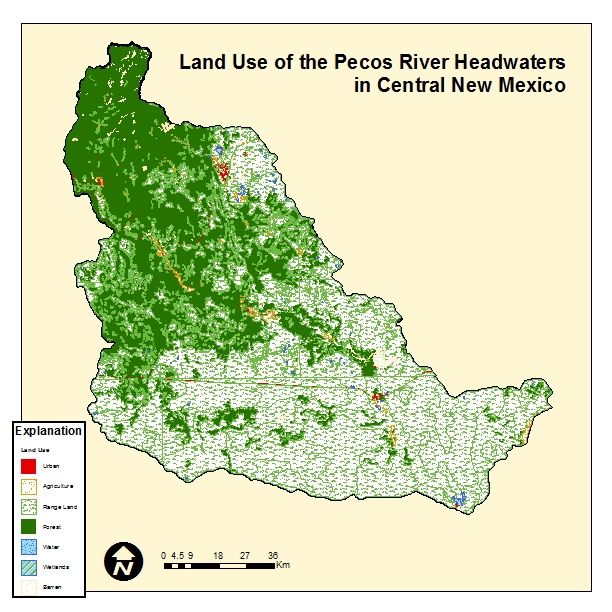
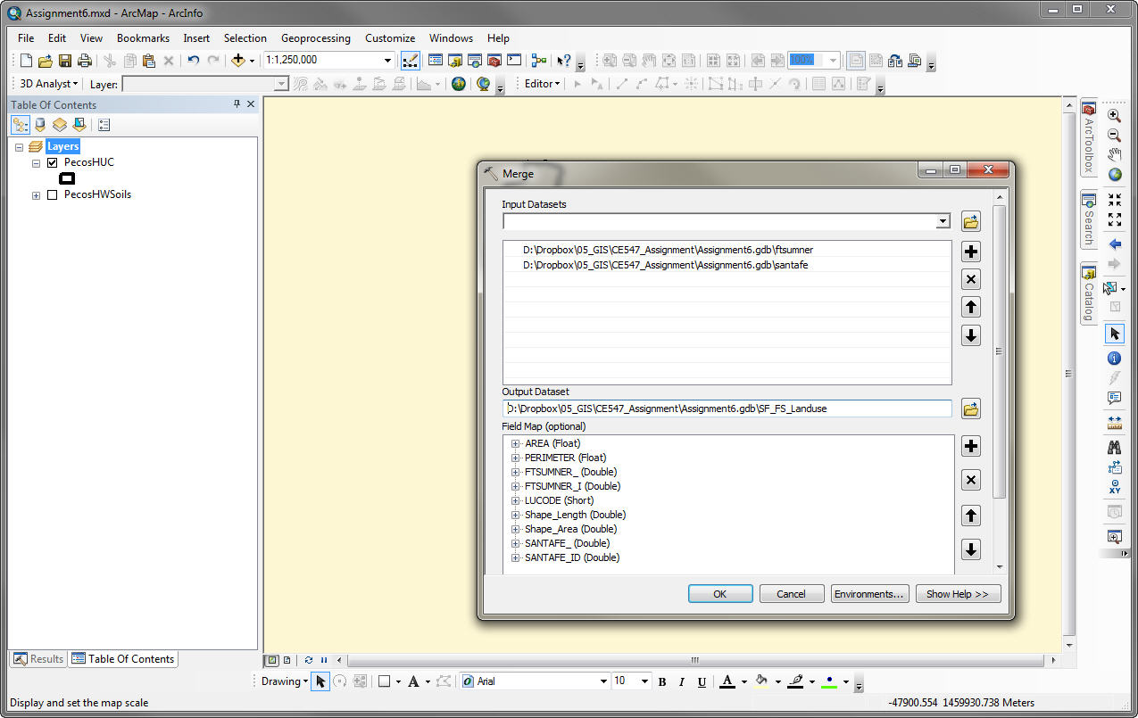
Land use files are available from the USGS ftp site and from the EPA ftp site. Additionally, EDAC makes land use files available. There are a total of 23 coverages to make up the state of New Mexico using the 1986 dataset. Two coverages are required for the headwaters of the Pecos: Ft Sumner and Santa Fe. You will need to download these from rgis.unm.edu. Extract the zips and import the layers to your gdb.
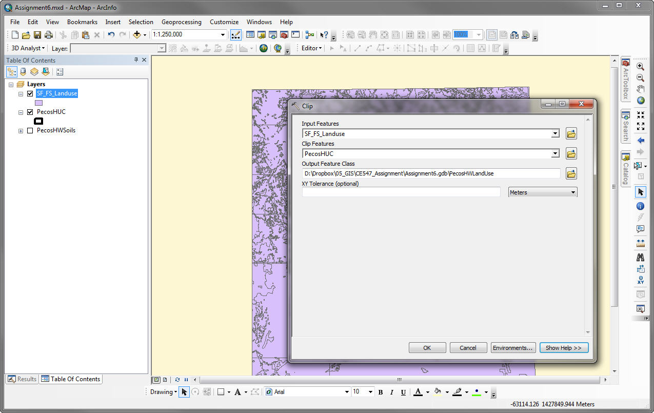
f) Merge and clip land use: Open the Merge toolbox, add the two land use shapefiles and set the output name. When new the layer is added to map, clip the land use to the PecosHUC.
These files use an
Anderson Land Use Code classification system, in which major land
use types are broken out into 9 categories:
1 = urban
2 = agriculture
3 = rangeland
4 = forest
5 = water
6 = wetlands
7 = barren land
8 = tundra
9 = ice and snow.
The second digit
distinguishes subcategories of these principal categories, e.g.
11 = urban residential
12 = urban commercial
13 = urban industrial, etc.
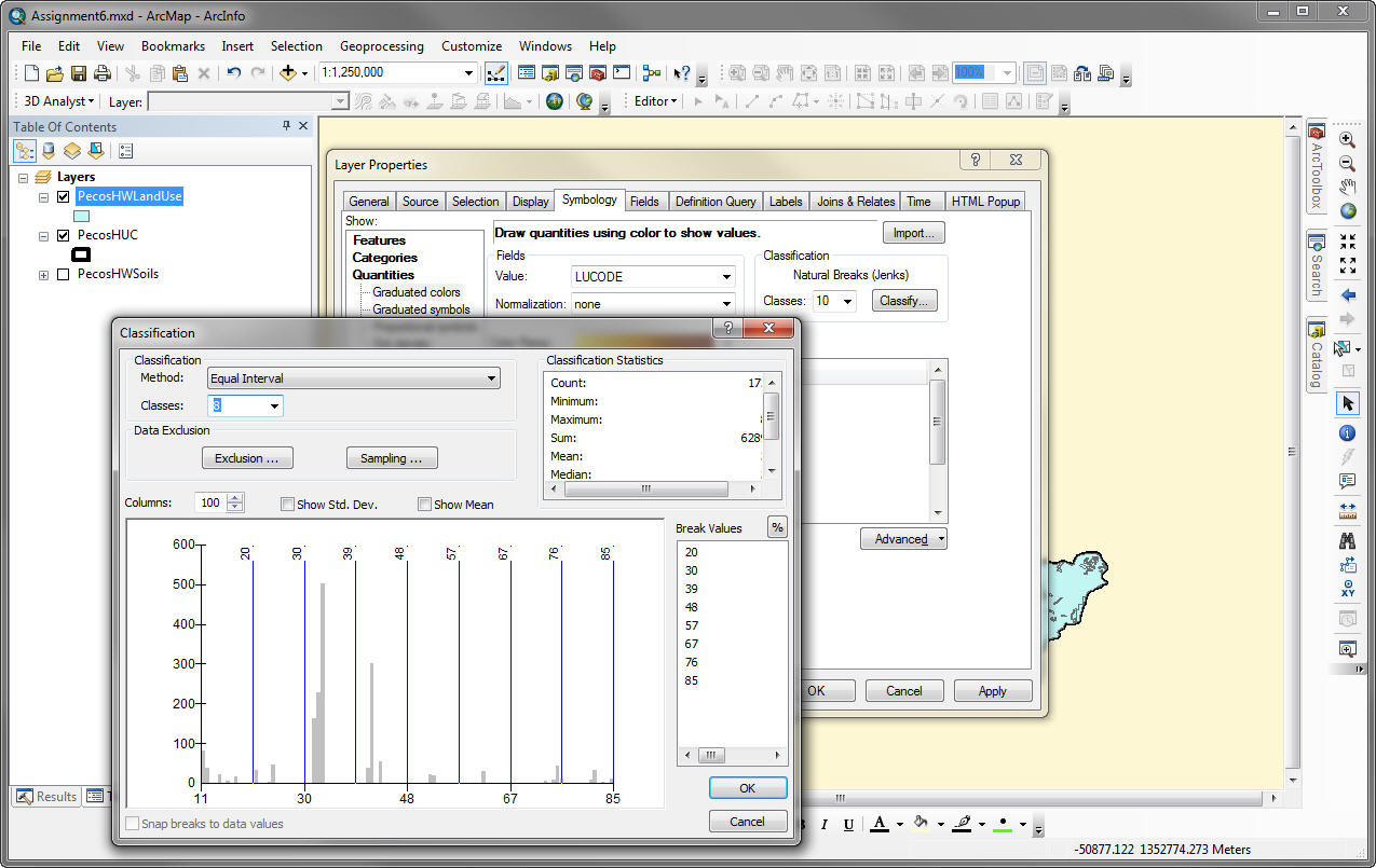
g) Change symbology: This land use classification for the United States was made in the late 1970's and land use has changed in the years since then, particularly as cities have grown. But, the LULC files are still the standard land use classification of the United States taken as a whole. Change the symbology of the layers so that they show the Anderson Land Use codes. Below, I am changing the symbology for Fort Sumner. I’m classifying by LUCODE. I switched the Classification Method to Equal Interval with 8 classes and then manually entered the Break Values.
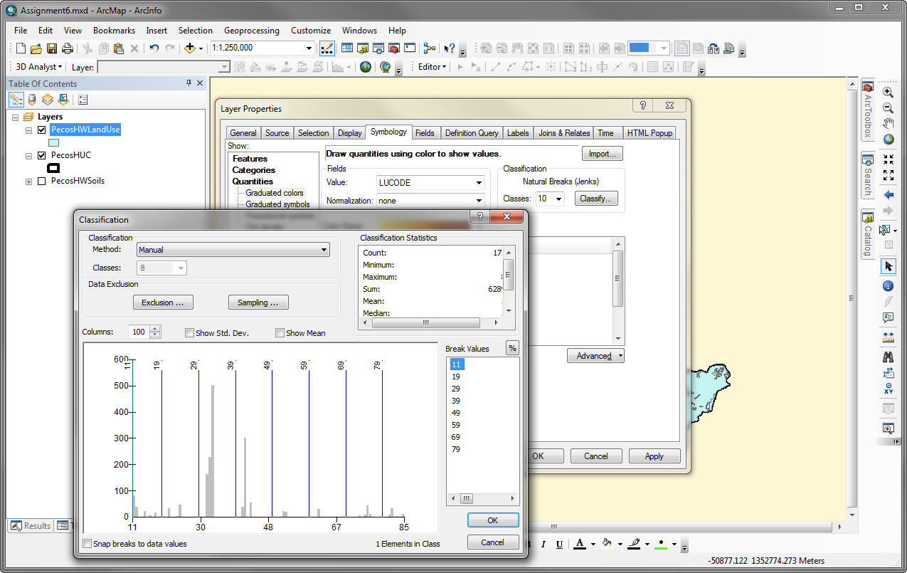
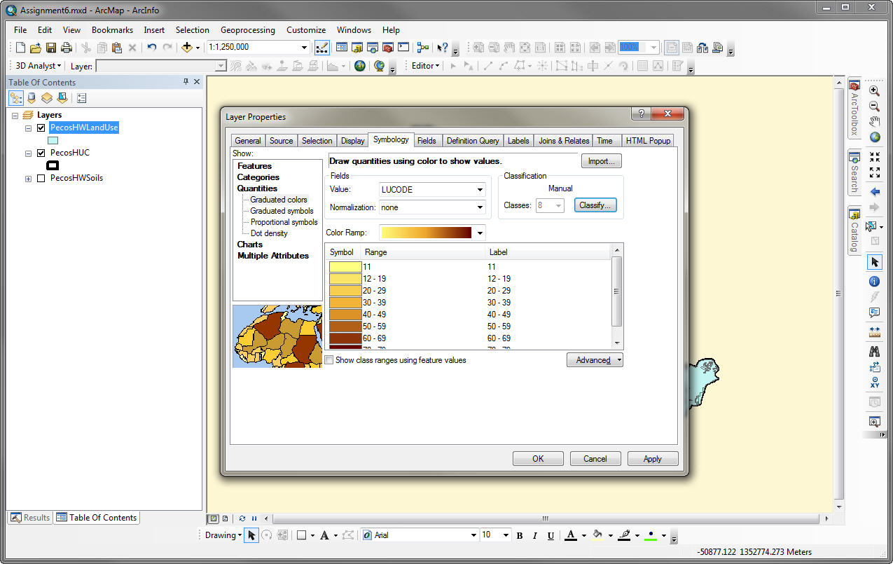
h) Change classification: Once I entered the break values as shown below, the classification method changed to Manual.
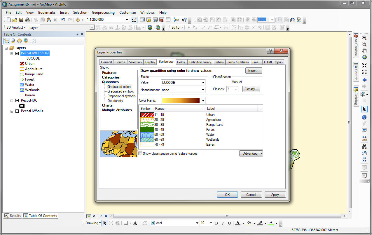
i) Adjust labels and colors: Next, you should change your labels and colors appropriately.
Look at the attribute table for your new shapefile. You have both soils information and land use information. It would not be too difficult to go a step further and get curve number (CN) information (something some might do for their project).
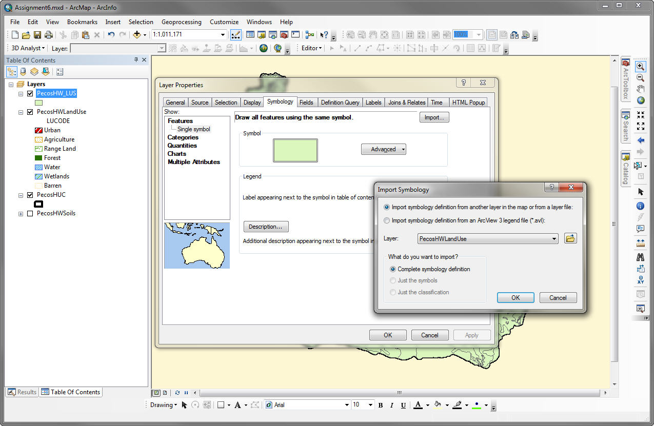
j) Import symbology: It would be nice for the new intersected layer to have the same symbology as your land use layer. Instead of taking the time to set each land use type you can simply import the symbology from the PecosHWLandUSe layer.
k) Export map: Create a couple of layouts and and them to your website.